Poisson approximations to the negative binomial distribution

This post is an introduction to the negative binomial distribution and a discussion of different ways of approximating the negative binomial distribution.

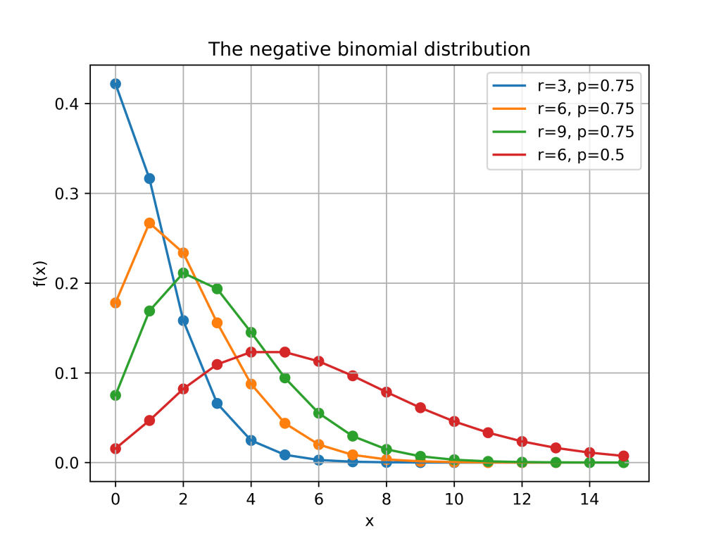
The negative binomial distribution describes the number of times a coin lands on tails before a certain number of heads are recorded. The distribution depends on two parameters p and r. The parameter p is the probability that the coin lands on heads and r is the number of heads. If X has the negative binomial distribution, then X = x means in the first x+r-1 tosses of the coin, there were r-1 heads and that toss number x+r was a head. This means that the probability that X=x is given by

\displaystyle{f(x) = \binom{x+r-1}{r-1}p^{r}\left(1-p\right)^x}

Here is a plot of the function f(x) for different values of r and p.

Poisson approximations

When the parameter r is large and p is close to one, the negative binomial distribution can be approximated by a Poisson distribution. More formally, suppose that r(1-p)=\lambda for some positive real number \lambda. If r is large then, the negative binomial random variable with parameters p and r, converges to a Poisson random variable with parameter \lambda. This is illustrated in the picture below where three negative binomial distributions with r(1-p)=5 approach the Poisson distribution with \lambda =5.

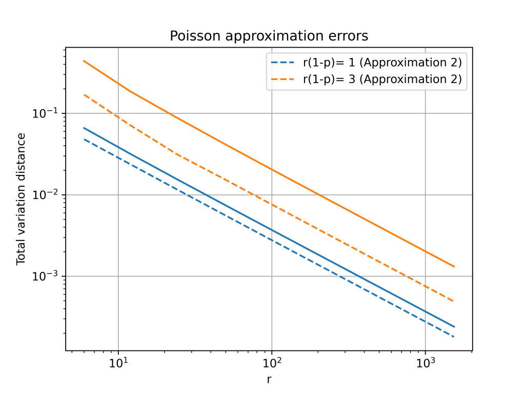
Total variation distance is a common way to measure the distance between two discrete probability distributions. The log-log plot below shows that the error from the Poisson approximation is on the order of 1/r and that the error is bigger if the limiting value of r(1-p) is larger.

It turns out that is is possible to get a more accurate approximation by using a different Poisson distribution. In the first approximation, we used a Poisson random variable with mean \lambda = r(1-p). However, the mean of the negative binomial distribution is r(1-p)/p. This suggests that we can get a better approximation by setting \lambda = r(1-p)/p.

The change from \lambda = r(1-p) to \lambda = r(1-p)/p is a small because p \approx 1. However, this small change gives a much better approximation, especially for larger values of r(1-p). The below plot shows that both approximations have errors on the order of 1/r, but the constant for the second approximation is much better.

Second order accurate approximation

It is possible to further improve the Poisson approximation by using a Gram–Charlier expansion. A Gram–Charlier approximation for the Poisson distribution is given in this paper.1 The approximation is

\displaystyle{f_{GC}(x) = P_\lambda(x) - \frac{1}{2}(1-p)\left((x-\lambda)P_\lambda(x)-(x-1-\lambda)P_\lambda(x-1)\right)},

where \lambda = \frac{k(1-p)}{p} as in the second Poisson approximation and P_\lambda(x) is the Poisson pmf evaluated at x.

The Gram–Charlier expansion is considerably more accurate than either Poisson approximation. The errors are on the order of 1/r^2. This higher accuracy means that the error curves for the Gram–Charlier expansion has a steeper slope.

  1. The approximation is given in equation (4) of the paper and is stated in terms of the CDF instead of the PMF. The equation also contains a small typo, it should say \frac{1}{2}q instead of \frac{1]{2}p. ↩︎

Leave a comment