michaelnhowes

Auxiliary variables sampler

The auxiliary variables sampler is a general Markov chain Monte Carlo (MCMC) technique for sampling from probability distributions with unknown normalizing constants [1, Section 3.1]. Specifically, suppose we have $n$ functions $f_i : \mathcal{X} \to (0,\infty)$ and we want to sample from the probability distribution $P(x) \propto \prod_{i=1}^n f_i(x).$ That is

$\displaystyle{ P(x) = \frac{1}{Z}\prod_{i=1}^n f_i(x)},$

where $Z = \sum_{x \in \mathcal{X}} \prod_{i=1}^n f_i(x)$ is a normalizing constant. If the set $\mathcal{X}$ is very large, then it may be difficult to compute $Z$ or sample from $P(x)$ . To approximately sample from $P(x)$ we can run an ergodic Markov chain with $P(x)$ as a stationary distribution. Adding auxiliary variables is one way to create such a Markov chain. For each $i \in \{1,\ldots,n\}$ , we add a auxiliary variable $U_i \ge 0$ such that

$\displaystyle{P(U \mid X) = \prod_{i=1}^n \mathrm{Unif}[0,f_i(X)]}.$

That is, conditional on $X$ , the auxiliary variables $U_1,\ldots,U_n$ are independent and $U_i$ is uniformly distributed on the interval $[0,f_i(X)]$ . If $X$ is distributed according to $P$ and $U_1,\ldots,U_n$ have the above auxiliary variable distribution, then

$\displaystyle{P(X,U) =P(X)P(U\mid X)\propto \prod_{i=1}^n f_i(X) \frac{1}{f_i(X)} I[U_i \le f(X_i)] = \prod_{i=1}^n I[U_i \le f(X_i)]}.$

This means that the joint distribution of $(X,U)$ is uniform on the set

$\widetilde{\mathcal{X}} = \{(x,u) \in \mathcal{X} \times (0,\infty)^n : u_i \le f(x_i) \text{ for all } i\}.$

Put another way, suppose we could jointly sample $(X,U)$ from the uniform distribution on $\widetilde{\mathcal{X}}$ . Then, the above calculation shows that if we discard $U$ and only keep $X$ , then $X$ will be sampled from our target distribution $P$ .

The auxiliary variables sampler approximately samples from the uniform distribution on $\widetilde{\mathcal{X}}$ is by using a Gibbs sampler. The Gibbs samplers alternates between sampling $U'$ from $P(U \mid X)$ and then sampling $X'$ from $P(X \mid U')$ . Since the joint distribution of $(X,U)$ is uniform on $\widetilde{\mathcal{X}}$ , the conditional distributions $P(X \mid U)$ and $P(U \mid X)$ are also uniform. The auxiliary variables sampler thus transitions from $X$ to $X'$ according to the two step process

Independently sample $U_i$ uniformly from $[0,f_i(X)]$ .
Sample $X'$ uniformly from the set $\{x \in \mathcal{X} : f_i(x) \ge u_i \text{ for all } i\}$ .

Since the auxiliary variables sampler is based on a Gibbs sampler, we know that the joint distribution of $(X,U)$ will converge to the uniform distribution on $\mathcal{X}$ . So when we discard $U$ , the distribution of $X$ will converge to the target distribution $P$ !

Auxiliary variables in practice

To perform step 2 of the auxiliary variables sampler we have to be able to sample uniformly from the sets

$\mathcal{X}_u = \{x \in \mathcal{X}:f_i(x) \ge u_i \text{ for all } i\}.$

Depending on the nature of the set $\mathcal{X}$ and the functions $f_i$ , it might be difficult to do this. Fortunately, there are some notable examples where this step has been worked out. The very first example of auxiliary variables is the Swendsen-Wang algorithm for sampling from the Ising model [2]. In this model it is possible to sample uniformly from $\mathcal{X}_u$ . Another setting where we can sample exactly is when $\mathcal{X}$ is the real numbers $\mathcal{R}$ and each $f_i$ is an increasing function of $x$ . This is explored in [3] where they apply auxiliary variables to sampling from Bayesian posteriors.

There is an alternative to sampling exactly from the uniform distribution on $\mathcal{X}_u$ . Instead of sampling $X'$ uniformly from $\mathcal{X}_u$ , we can run a Markov chain from the old $X$ that has the uniform distribution as a stationary distribution. This approach leads to another special case of auxiliary variables which is called “slice sampling” [4].

References

[1] Andersen HC, Diaconis P. Hit and run as a unifying device. Journal de la societe francaise de statistique & revue de statistique appliquee. 2007;148(4):5-28. http://www.numdam.org/item/JSFS_2007__148_4_5_0/
[2] Swendsen RH, Wang JS. Nonuniversal critical dynamics in Monte Carlo simulations. Physical review letters. 1987 Jan 12;58(2):86. https://journals.aps.org/prl/abstract/10.1103/PhysRevLett.58.86
[3] Damlen P, Wakefield J, Walker S. Gibbs sampling for Bayesian non‐conjugate and hierarchical models by using auxiliary variables. Journal of the Royal Statistical Society: Series B (Statistical Methodology). 1999 Apr;61(2):331-44. https://rss.onlinelibrary.wiley.com/doi/abs/10.1111/1467-9868.00179
[4] Neal RM. Slice sampling. The annals of statistics. 2003 Jun;31(3):705-67. https://projecteuclid.org/journals/annals-of-statistics/volume-31/issue-3/Slice-sampling/10.1214/aos/1056562461.full

Fibonacci series

In “Probabilizing Fibonacci Numbers” Persi Diaconis recalls asking Ron Graham to help him make his undergraduate number theory class more fun. Persi asks about the chance a Fibonacci number is even and whether infinitely many Fibonacci numbers are prime. After answering “1/3” and “no one knows” to Persi’s questions, Ron suggests giving the undergrads the following problem:

$\displaystyle{\sum_{n=1}^\infty \frac{F_n}{10^n} = \frac{10}{89}}$

While no longer an undergrad, I found the problem fun to solve and wanted to work out the general pattern. Above $F_n$ is the $n$ th Fibonacci number. So $F_0=0,F_1=1$ and $F_{n} = F_{n-1} + F_{n-2}$ for $n \ge 2$ . Ron’s infinite series can be proved using the recurrence relation for the Fibonacci numbers and the general result is that for any $c > \varphi = \frac{1+\sqrt{5}}{2} \approx 1.618$

$\displaystyle{\sum_{n=1}^\infty \frac{F_n}{c^n} = \frac{c}{c^2-c-1}}.$

To see why, first note that $F_n \approx \varphi^n/\sqrt{5}$ so the sum does converge for $c>\varphi$ . Let $x = \sum_{n=1}^\infty \frac{F_n}{c^n}$ be the value of the sum. If we multiply $x$ by $c^2$ , then we get

$\displaystyle{c^2 x = \frac{c^2F_1}{c} + \sum_{n=2}^\infty \frac{F_n}{c^{n-2}} = c + \sum_{n=2}^\infty \frac{F_{n-1}}{c^{n-2}} + \sum_{n=2}^\infty \frac{F_{n-2}}{c^{n-2}} .}$

But

$\displaystyle{\sum_{n=2}^\infty \frac{F_{n-2}}{c^{n-2}}=x}$ and $\displaystyle{\sum_{n=2}^\infty \frac{F_{n-1}}{c^{n-2}}=cx}$ .

Together this implies that $c^2 x = c+cx+x$ and so

$\displaystyle{\sum_{n=1}^\infty \frac{F_n}{c^n} = x = \frac{c}{c^2-c-1}.}$

Generating functions

The above calculation is closely related to the generating function of the Fibonacci numbers. The generating function of the Fibonacci numbers is the function $f(z)$ given by

$\displaystyle{f(z) = \sum_{n=1}^\infty F_n z^n.}$

If we let $z = c^{-1}$ , then by Ron’s exercise

$\displaystyle{f(z) = \frac{c}{c^2-c-1}=\frac{z^{-1}}{z^{-2}-z^{-1}-1} = \frac{z}{1-z-z^2},}$

for $z < \varphi^{-1}$ . So solving Ron’s exercise is equivalent to finding the generating function of the Fibonacci numbers!

Other sums

In “Probabilizing Fibonacci Numbers”, Ron also suggests getting the undergrads to add up $\sum_{k=0}^\infty \frac{1}{F_{2^k}}$ . I leave this sum for another blog post!

The fast Fourier transform as a matrix factorization

The discrete Fourier transform (DFT) is a mapping from $\mathbb{C}^n$ to $\mathbb{C}^n$ . Given a vector $u \in \mathbb{C}^n$ , the discrete Fourier transform of $u$ is another vector $U \in \mathbb{C}^n$ given by,

$\displaystyle{U_k = \sum_{j=0}^{n-1} \exp\left(-2 \pi i kj/m\right)u_j}.$

If we let $\omega_n = \exp\left(-2 \pi i /m\right)$ , then $U$ can be written more compactly as

$\displaystyle{U_k = \sum_{j=0}^{n-1} \omega^{kj}_n u_j }.$

The map from $u$ to $U$ is linear and can therefor be represented as multiplication by an $n \times n$ matrix $D$ . Looking at the equation above, we can see that if we set $D_{kj} = \omega^{kj}_n$ and use $0$ -indexing, then,

$U = Du.$

This suggests that calculating the vector $U = Du$ would require roughly $n^2$ operations. However, the famous fast Fourier transform shows that $U$ can be computed in roughly $n\log_2(n)$ operations. There are many derivations of the fast Fourier transform but I wanted to focus on one which is based on factorizing the matrix $D$ into sparse matrices.

Matrix factorizations

A factorization of a matrix $A$ is a way of writing $A$ as a product of matrices $A = A_L\cdots A_2A_1$ where typically $L$ is $2$ or $3$ . Matrix factorizations can tell us information about the matrix $A$ . For example, the singular value decomposition tells us the spectral norm and singular vectors $A$ (and lots more). Other matrix factorizations can help us compute things related to the matrix $A$ . The QR decomposition helps us solve least-squares problems and the LU factorization let us invert $A$ in (almost) the same amount of time it takes to solve the equation $Ax = b$ .

Each of the factorizations above applied to arbitrary matrices. Every possible matrix has an singular value decomposition and a QR factorization. Likewise all square matrices have an LU factorization. The DFT matrix $D$ has a factorization which most matrices other matrices do not. This factorization lets us write $D = D_L\cdots D_2D_1$ where each matrix $D_l$ is sparse.

Sparse matrices

A matrix $A$ is sparse if many of the entries of $A$ are zero. There isn’t a precise definition of “many”. A good heuristic is that if $A$ has size $m$ by $n$ , then $A$ is sparse if the number of non-zero entries is of the order $m$ or $n$ . In contrast, a dense matrix is one where the number of non-zero entries is of the same order of $mn$ .

The structure of sparse matrices makes them especially nice to work with. They take up a lot less memory and they are quicker to compute with. If $A \in \mathbb{C}^{m \times n}$ has only $k$ non-zero elements, then for any vector $x \in \mathbb{C}^n$ , the matrix-vector product $Ax$ can be computed in order $k$ operations. If $k$ is much less than $mn$ , then this can be a huge speed up.

This shows why a sparse factorization of the DFT matrix $D$ will give a fast way of calculating $Du$ . Specifically, suppose that we have $D = D_L \cdots D_2D_1$ and each matrix $D_l$ has just $k_l$ non-zero entries. Then, for any vector $u \in \mathbb{C}^n$ , we can compute $U= Du=D_L \cdots D_2 D_1 u$ in stages. First we multiply $u$ by $D_1$ to produce $u^{(1)}$ . The output $u^{(1)}$ is then multiplied by $D_2$ to produce $u^{(2)}$ . We continue in this way until we finally multiply $u^{(L-1)}$ by $D_L$ to produce $u = D_L u^{(L-1)}$ . The total computation cost is of the order $k_1 + k_2 + \cdots + k_L$ which can be drastically less than $n^2$ .

The DFT factorization

We’ll now show that $D$ does indeed have a sparse matrix factorization. To avoid some of the technicalities, we’ll assume that $n$ is a power of $2$ . That is, $n = 2^m$ for some $m$ . Remember that the discrete Fourier transform of $u$ is the vector $U$ given by

$\displaystyle{U_k = \sum_{j=0}^{n-1} \omega^{jk}_n u_j},$

where $\omega_n = \exp(-2\pi i/n)$ . The idea behind the fast Fourier transform is to split the above sum into two terms. One where we add up the even values of $j$ and one where we add up the odd values of $j$ . Specifically,

$\displaystyle{U_k = \sum_{j=0, \text{j even }}^{n-1} \omega_n^{jk} u_j + \sum_{j = 0, j \text{ odd}}^{n-1} \omega_n^{jk}u_j = \sum_{j=0}^{n/2 - 1} \omega^{2jk}_n u_{2j} + \sum_{j=0}^{n/2-1} \omega^{(2j+1)k}_n u_{2j+1}}$

We’ll now look at each of these sums separately. In the first sum, we have terms of the form $\omega^{2 jk}_n$ , these can by rewritten as follows,

$\omega^{2 jk}_n = \exp(-2 \pi i /n)^{2 jk} = \exp(-2 \pi i 2/n)^{jk} = \exp(-2 \pi i /(n/2))^{jk} = \omega_{n/2}^{jk}$ .

We can also use this result to rewrite the terms $\omega^{(2j+1)k}_n$ ,

$\omega^{(2j+1)k}_n = \omega_n^k\omega^{2jk}_n = \omega_n^k \omega^{jk}_{n/2}.$

If we plug both of these back into the expression for $U = Du$ , we get

$\displaystyle{U_k = \sum_{j=0}^{n/2 - 1} \omega_{n/2}^{jk} u_{2j} + \sum_{j=0}^{n/2-1} \omega_n^k \omega_{n/2}^{jk} u_{2j+1} = \sum_{j=0}^{n/2-1} \omega_{n/2}^{jk} u_{2j} + \omega_n^k \sum_{j=0}^{n/2-1}\omega_{n/2}^{jk} u_{2j+1}. }$

This shows that the Fourier transform of the $n$ -dimensional vector $u$ can be done by computing and combining the Fourier transforms of the $n/2$ -dimensional vectors. One of these vectors contain the even indexed elements of $u$ and the others contain the odd indexed elements of $u$ .

There is one more observation that we need. If $k$ is between $n/2$ and $n-1$ , then we can simplify the above expression for $U_k$ . Specifically, if we set $k'=k-n/2$ , then

$\omega_{n/2}^{jk} = \omega_{n/2}^{j(n/2+k')} = \omega_{n/2}^{jn/2}\omega_{n/2}^{jk'} = \exp(-2\pi i (n/2)/(n/2))^j \omega_{n/2}^{jk'} = \omega_{n/2}^{jk'}.$

If we plug this into the above formula for $U_k$ , then we get

$\displaystyle{U_k = \sum_{j=0}^{n/2-1} \omega_{n/2}^{j(k-n/2)} u_{2j} + \omega_n^k \sum_{j=0}^{n/2-1}\omega_{n/2}^{j(k-n/2)} u_{2j+1}}$ for $k = n/2, n/2+1,\ldots, n-1$ .

This reduces the computation since there are some computations we only have to do once but can use twice. The algebra we did above shows that we can compute the discrete Fourier transform of $u \in \mathbb{C}^n$ in the following step.

Form the vectors $u^{\text{even}} = (u_0,u_2,\ldots,u_{n-2}) \in \mathbb{C}^{n/2}$ and $u^{\text{odd}} = (u_1,u_3,\ldots,u_{n-1}) \in \mathbb{C}^{n/2}$ .
Calculate the discrete Fourier transforms of $u^{\text{even}}$ and $u^{\text{odd}}$ . This gives two vector $U^{\text{even}}, U^{\text{odd}} \in \mathbb{C}^{n/2}$ .
Compute $U \in \mathbb{C}^n$ by,

$\displaystyle{U_k = \begin{cases} U^{\text{even}}_k + \omega_n^k U^{\text{odd}}_k & \text{for } k = 0,1,\ldots, n/2-1,\\ U^{\text{even}}_{k-n/2}+\omega_n^k U^{\text{odd}}_{k-n/2} &\text{for } k=n/2,n/2+1,\ldots,n-1 \end{cases}}$

The steps above break down computing $U=Du$ into three simpler steps. Each of these simpler steps are also linear maps and can therefore be written as multiplication by a matrix. If we call these matrices $D_1,D_2$ and $D_3$ , then

The matrix $D_1$ maps $u$ to $\begin{bmatrix} u^{\text{even}} \\ u^{\text{odd}}\end{bmatrix}$ . That is

$D_1 = \begin{bmatrix} 1&0&0&0&\cdots&0&0\\0&0&1&0&\cdots &0&0 \\\vdots& \vdots &\vdots & \vdots & \ddots & \vdots & \vdots \\0&0&0&0&\cdots&1&0 \\ 0&1&0&0&\cdots&0&0 \\ 0&0&0&1&\cdots&0&0 \\ \vdots&\vdots &\vdots & \vdots & \ddots & \vdots & \vdots \\ 0&0&0&0&\cdots&0&1\end{bmatrix} \in \mathbb{C}^{n \times n}.$

The matrix $D_2$ is block-diagonal and each block is the $n/2$ -dimensional discrete Fourier transformation matrix. That is

$D_2 = \begin{bmatrix}D^{(n/2)} & 0\\ 0 & D^{(n/2)}\end{bmatrix}\in \mathbb{C}^{n \times n},$

where $D^{(n/2)}$ is given by $D^{(n/2)}_{jk} = \omega_{n/2}^{jk}$ .

The matrix $D_3$ combines two $n/2$ -vectors according to the formula in step 3 above,

$D_3 = \begin{bmatrix} 1&0&\cdots & 0 & \omega_n^0 & 0 & \cdots & 0\\ 0&1&\cdots&0 &0& \omega_n^1&\cdots & 0\\ \vdots & \vdots & \ddots & \vdots & \vdots& \vdots &\ddots&\vdots\\ 0&0&\cdots & 1 & 0 & 0 & \cdots & \omega_n^{n/2-1}\\1&0&\cdots & 0 & \omega_n^{n/2} & 0 & \cdots & 0\\ 0&1&\cdots&0 &0& \omega_n^{n/2+1}&\cdots & 0\\ \vdots & \vdots & \ddots & \vdots & \vdots& \vdots &\ddots&\vdots\\ 0&0&\cdots & 1 & 0 & 0 & \cdots & \omega_n^{n-1}\end{bmatrix}\in \mathbb{C}^{n \times n}$

The three-step procedure above for calculating $U=Du$ is equivalent to iteratively multiplying by $D_1$ , then $D_2$ and the finally by $D_3$ . Another way of saying this is that $D=D_3D_2D_1$ is a matrix factorization!

From the definitions, we can see that each of the matrices $D_1,D_2$ and $D_3$ have a lot of zeros. Specifically, $D_1$ has just $n$ non-zero entries (one in each row), $D_2$ has $2(n/2)^2$ non-zero entries (two blocks of $n/2 \times n/2$ non-zeros) and $D_3$ has $2n$ non-zero entries (two in each row). This means that the product $U=D_3D_2D_1u$ can be computed in roughly

$n+2(n/2)^2 + 2n = 3n+2(n/2)^2,$

operations. This is far away from the $n\log_2(n)$ operations promised at the start of this blog post. However, the matrix $D_2$ contains two copies of the $n/2 \times n/2$ discrete Fourier transform matrix. This means we could apply the exact same argument to the $n/2 \times n/2$ matrix $D^{(n/2)}$ . This lets us replace $(n/2)^2$ with $\frac{3}{2}n + 2(n/4)^2$ . This brings the number of operations down to

$3n+2\left(\frac{3}{2}n + 2(n/4)^2\right) = 6n + 4(n/4)^2.$

We can again keep going! If we recall that $n=2^m$ , then we get to repeat the proccess $m$ times in total giving approximately,

$3mn + 2^m = 3\log_2(n)n+n,$ operations.

So by using lots of sparse matrices, we can compute $U=Du$ in $\approx n\log_2(n)$ operations instead of $\approx n^2$ operations.

Doing Calvin’s homework

Growing up, my siblings and I would read a lot of Bill Watterson’s Calvin and Hobbes. I have fond memories of spending hours reading and re-reading our grandparents collection during the school holidays. The comic strip is witty, heartwarming and beautifully drawn.

Recently, I came across this strip online

Originally published Feb 5th, 1990 by Bill Watterson. All creative credit goes to Bill. You can read the rest of the story arc here: https://www.gocomics.com/calvinandhobbes/1990/02/05

Seeing Calvin take this test took me back to those school holidays. I remember grabbing paper and a pencil to work out the answer (I also remember getting teased by those previously mentioned siblings). Reading the strip years later, I realized there’s a neat way to work out the answer without having to write much down. Here’s the question again,

Jack and Joe leave their homes at the same time and drive toward each other. Jack drives at 60 mph, while Joe drives at 30 mph. They pass each other in 10 minutes.

How far apart were Jack and Joe when they started?

It can be hard to think about Jack and Joe traveling at different speeds. But we can simplify the problem by thinking from Joe’s perspective or frame of reference. From Joe’s frame of reference, he is staying perfectly still but Jack is zooming towards him at $30+60=90$ mph. Jack reaches Joe in 10 minutes which is one sixth of an hour. This means that the initial distance between them must have been $90 \times 1/6 = 15$ miles.

It’s not as creative as Calvin’s private eye approach but at least Susie and I got the same answer.

Originally published Feb 10th, 1990 by Bill Watterson. Again all creative credit goes to Bill. https://www.gocomics.com/calvinandhobbes/1990/02/10

Bernoulli’s inequality and probability

Suppose we have independent events $E_1,E_2,\ldots,E_m$ , each of which occur with probability $1-\varepsilon$ . The event that all of the $E_i$ occur is $E = \bigcap_{i=1}^m E_i$ . By using independence we can calculate the probability of $E$ ,

$P(E) = P\left(\bigcap_{i=1}^m E_i\right) = \prod_{i=1}^m P(E_i) = (1-\varepsilon)^m.$

We could also get a lower bound on $P(E)$ by using the union bound. This gives,

$P(E) = 1-P(E^c) = 1-P\left(\bigcup_{i=1}^m E_i^c\right) \ge `1-\sum_{i=1}^m P(E_i^c) = 1-m\varepsilon.$

We can therefore conclude that $(1-\varepsilon)^m \ge 1-m\varepsilon$ . This is an instance of Bernoulli’s inequality. More generally, Bernoulli’s inequality states that

$(1+x)^m \ge 1+mx,$

for all $x \ge -1$ and $m \ge 1$ . This inequality states the red line is always underneath the black curve in the below picture. For an interactive version of this graph where you can change the value of $m$ , click here.

Our probabilistic proof only applies to that case when $x = -\varepsilon$ is between $-1$ and $0$ and $m$ is an integer. The more general result can be proved by using convexity. For $m \ge 1$ , the function $f(x) = (1+x)^m$ is convex on the set $x > -1$ . The function $g(x) = 1+mx$ is the tangent line of this function at the point $x=0$ . Convexity of $f(x)$ means that the graph of $f(x)$ is always above the tangent line $g(x)$ . This tells us that $(1+x)^m \ge 1+mx$ .

For $m$ between $0$ and $1$ , the function $(1+x)^m$ is no longer convex but actually concave and the inequality reverses. For $m \le 0$ , $(1+x)^m$ becomes concave again. These two cases are visualized below. In the first picture $m = 0.5$ and the red line is above the black one. In the second picture $m = -1$ and the black line is back on top.

Solving a system of equations vs inverting a matrix

I used to have trouble understanding why inverting an $n \times n$ matrix required the same order of operations as solving an $n \times n$ system of linear equations. Specifically, if $A$ is an $n\times n$ invertible matrix and $b$ is a length $n$ vector, then computing $A^{-1}$ and solving the equation $Ax = b$ can both be done in $O(n^3)$ floating point operations (flops). This surprised me because naively computing the columns of $A^{-1}$ requires solving the $n$ systems of equations

$Ax = e_1, Ax=e_2,\ldots, Ax = e_n,$

where $e_1,e_2,\ldots, e_n$ are the standard basis vectors. I thought this would mean that calculating $A^{-1}$ would require roughly $n$ times as many flops as solving a single system of equations. It was only in a convex optimization lecture that I realized what was going on.

To solve a single system of equations $Ax = b$ , we first compute a factorization of $A$ such as the LU factorization. Computing this factorization takes $O(n^3)$ flops but once we have it, we can use it solve any new system with $O(n^2)$ flops. Now to solve $Ax=e_1,Ax=e_2,\ldots,Ax=e_n$ , we can simply factor $A$ once and the perform $n$ solves using the factorization each of which requires an addition $O(n^2)$ flops. The total flop count is then $O(n^3)+nO(n^2)=O(n^3)$ . Inverting the matrix requires the same order of flops as a single solve!

Of course, as John D Cook points out: you shouldn’t ever invert a matrix. Even if inverting and solving take the same order of flops, inverting is still more computational expensive and requires more memory.

Concavity of the squared sum of square roots is about an interesting homework problem from the same convex optimization course.

Braids and the Yang-Baxter equation

I recently gave a talk on the Yang-Baxter equation. The focus of the talk was to state the connection between the Yang-Baxter equation and the braid relation. This connection comes from a system of interacting particles. In this post, I’ll go over part of my talk. You can access the full set of notes here.

Interacting particles

Imagine two particles on a line, each with a state that can be any element of a set $\mathcal{X}$ . Suppose that the only way particles can change their states is by interacting with each other. An interaction occurs when two particles pass by each other. We could define a function $F : \mathcal{X} \times \mathcal{X} \to \mathcal{X} \times \mathcal{X}$ that describes how the states change after interaction. Specifically, if the first particle is in state $x$ and the second particle is in state $y$ , then their states after interacting will be

$F(x,y) = (F_a(x,y), F_b(x,y)) = (\text{new state of particle 1}, \text{new state of particle 2}),$

where $F_a,F_b : \mathcal{X} \times \mathcal{X} \to \mathcal{X}$ are the components of $F$ . Recall that the particles move past each other when they interact. Thus, to keep track of the whole system we need an element of $\mathcal{X} \times \mathcal{X}$ to keep track of the states and a permutation $\sigma \in S_2$ to keep track of the positions.

Three particles

Now suppose that we have $3$ particles labelled $1,2,3$ . As before, each particle has a state in $\mathcal{X}$ . We can thus keep track of the state of each particle with an element of $\mathcal{X}^3$ . The particles also have a position which is described by a permutation $\sigma \in S_3$ . The order the entries of $(x,y,z) \in \mathcal{X}^3$ corresponds to the labels of the particles not their positions. A possible configuration is shown below:

Three dots. The dots are labelled above 1, 3, 2 and labelled below x, z, y. — A possible configuration of the three particles. The above configuration is escribed as having states $(x,y,z) \in \mathcal{X}^3$ and positions $132 \in S_3$ .

A possible configuration of the three particles. The above configuration is escribed as having states $(x,y,z) \in \mathcal{X}^3$ and positions $132 \in S_3$ .

As before, the particles can interact with each other. However, we’ll now add the restriction that the particles can only interact two at a time and interacting particles must have adjacent positions. When two particles interact, they swap positions and their states change according to $F$ . The state and position of the remaining particle is unchanged. For example, in the above picture we could interact particles $1$ and $3$ . This will produce the below configuration:

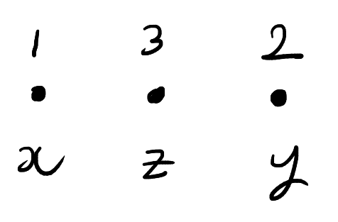
The new configuration after interacting particles $1$ and $3$ in the first diagram. The configuration is now described by the states $F_{13}(x,y,z) \in \mathcal{X}^3$ and the permutation $312 \in S_3$ .

To keep track of how the states of the particles change over time we will introduce three functions from $\mathcal{X}^3$ to $\mathcal{X}^3$ . These functions are $F_{12},F_{13},F_{23}$ . The function $F_{ij}$ is given by applying $F$ to the $i,j$ coordinates of $(x,y,z)$ and acting by the identity on the remaining coordinate. In symbols,

$F_{12}(x,y,z) = (F_a(x,y), F_b(x,y), z),$
$F_{13}(x,y,z) = (F_a(x,z), y, F_b(x,z)),$
$F_{23}(x,y,z) = (x, F_a(y,z), F_b(y,z)).$

The function $F_{ij}$ exactly describes how the states of the three particles change when particles $i$ and $j$ interact. Now suppose that three particles begin in position $123$ and states $(x,y,z)$ . We cannot directly interact particles $1$ and $3$ since they are not adjacent. We have to pass first pass one of the particles through particle $2$ . This means that there are two ways we can interact particles $1$ and $3$ . These are illustrated below.

The two ways of passing through particle 2 to interact particles 2 and 3.

In the top chain of interactions, we first interact particles $2$ and $3$ . In this chain of interactions, the states evolve as follows:

$(x,y,z) \to F_{23}(x,y,z) \to F_{13}(F_{23}(x,y,z)) \to F_{12}(F_{13}(F_{23}(x,y,z))).$

In the bottom chain of interactions, we first interact particles $1$ and $2$ . On this chain, the states evolve in a different way:

$(x,y,z) \to F_{12}(x,y,z) \to F_{13}(F_{12}(x,y,z)) \to F_{23}(F_{13}(F_{12}(x,y,z))).$

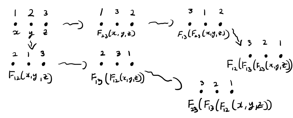
Note that after both of these chains of interactions the particles are in position $321$ . The function $F$ is said to solve the Yang–Baxter equation if two chains of interactions also result in the same states.

Definition: A function $F : \mathcal{X} \times \mathcal{X} \to \mathcal{X} \times \mathcal{X}$ is a solution to the set theoretic Yang–Baxter equation if,

$F_{12}\circ F_{13} \circ F_{23} = F_{23} \circ F_{13} \circ F_{12}.$

This equation can be visualized as the “braid relation” shown below. Here the strings represent the three particles and interacting two particles corresponds to crossing one string over the other.

Here are some examples of solutions to the set theoretic Yang-Baxter equation,

The identity on $\mathcal{X} \times \mathcal{X}$ .
The swap map, $(x,y) \mapsto (y,x)$ .
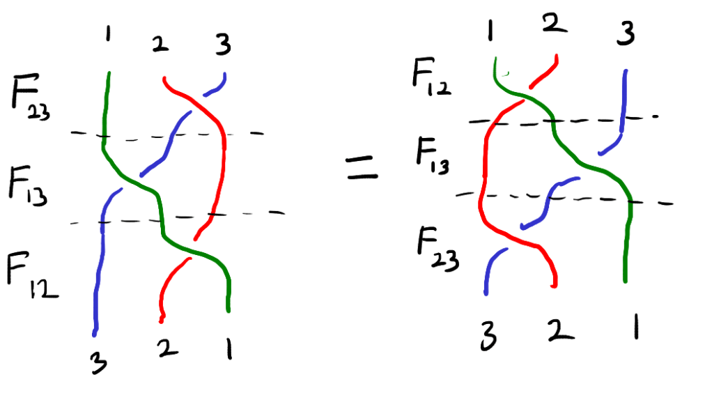
If $f,g : \mathcal{X} \to \mathcal{X}$ commute, then the function $(x,y) \to (f(x), g(y))$ is a solution the Yang-Baxter equation.

In the full set of notes I talk about a number of extensions and variations of the Yang-Baxter equation. These include having more than three particles, allowing for the particle states to be entangle and the parametric Yang-Baxter equation.

Concavity of the squared sum of square roots

The $p$ -norm of a vector $x\in \mathbb{R}^n$ is defined to be:

$\displaystyle{\Vert x \Vert_p = \left(\sum_{i=1}^n |x_i|^p\right)^{1/p}}.$

If $p \ge 1$ , then the $p$ -norm is convex. When $0<p<1$ , this function is not convex and actually concave when all the entries of $x$ are non-negative. On a recent exam for the course Convex Optimization, we were asked to prove this when $p = 1/2$ . In this special case, the mathematics simplifies nicely.

When $p = 1/2$ , the $p$ -norm can be described as the squared sum of square roots. Specifically,

$\displaystyle{\Vert x \Vert_{1/2} = \left(\sum_{i=1}^n \sqrt{|x_i|} \right)^2}.$

Note that we can expand the square and rewrite the function as follows

$\displaystyle{\Vert x \Vert_{1/2} = \sum_{i=1}^n\sum_{k=1}^n\sqrt{\left|x_i\right|} \sqrt{|x_k|} =\sum_{i=1}^n\sum_{k=1}^n \sqrt{|x_ix_k|}}.$

If we restrict to $x \in \mathbb{R}^n$ with $x_i \ge 0$ for all $i$ , then this function simplifies to

$\displaystyle{\Vert x \Vert_{1/2} =\sum_{i=1}^n\sum_{k=1}^n \sqrt{x_ix_k}},$

which is a sum of geometric means. The geometric mean function $(u,v) \mapsto \sqrt{uv}$ is concave when $u,v \ge 0$ . This can be proved by calculating the Hessian of this function and verifying that it is negative semi-definite.

From this, we can conclude that each function $x \mapsto \sqrt{x_ix_k}$ is also concave. This is because $x \mapsto \sqrt{x_ix_k}$ is a linear function followed by a concave function. Finally, any sum of concave functions is also concave and thus $\Vert x \Vert_{1/2}$ is concave.

Hellinger distance

A similar argument can be used to show that Hellinger distance is a convex function. Hellinger distance, $d_H(\cdot,\cdot)$ is defined on pairs of probability distributions $p$ and $q$ on a common set $\{1,\ldots,n\}$ . For such a pair,

$\displaystyle{d_H(p,q) = \sum_{i=1}^n \left(\sqrt{p_i}-\sqrt{q_i}\right)^2},$

which certainly doesn’t look convex. However, we can expand the square and use the fact that $p$ and $q$ are probability distributions. This shows us that Helligener distance can be written as

$\displaystyle{d_H(p,q) = \sum_{i=1}^n p_i - 2\sum_{i=1}^n \sqrt{p_iq_i}+\sum_{i=1}^n q_i = 2 - 2\sum_{i=1}^n\sqrt{p_iq_i}}.$

Again, each function $(p,q) \mapsto \sqrt{p_iq_i}$ is concave and so the negative sum of such functions is convex. Thus, $d_H(p,q)$ is convex.

The course

As a final comment, I’d just like to say how much I am enjoying the class. Prof. Stephen Boyd is a great lecturer and we’ve seen a wide variety of applications in the class. I’ve recently been reading a bit of John D Cook’s blog and agree with all he says about the course here.

Log-sum-exp trick with negative numbers

Suppose you want to calculate an expression of the form

$\displaystyle{\log\left(\sum_{i=1}^n \exp(a_i) - \sum_{j=1}^m \exp(b_j)\right)},$

where $\sum_{i=1}^n \exp(a_i) > \sum_{j=1}^m \exp(b_j)$ . Such expressions can be difficult to evaluate directly since the exponentials can easily cause overflow errors. In this post, I’ll talk about a clever way to avoid such errors.

If there were no terms in the second sum we could use the log-sum-exp trick. That is, to calculate

$\displaystyle{\log\left(\sum_{i=1}^n \exp(a_i) \right)},$

we set $a=\max\{a_i : 1 \le i \le n\}$ and use the identity

$\displaystyle{a + \log\left(\sum_{i=1}^n \exp(a_i-a)\right) = \log\left(\sum_{i=1}^n \exp(a_i)\right)}.$

Since $a_i \le a$ for all $i =1,\ldots,n$ , the left hand side of the above equation can be computed without the risk of overflow. To calculate,

$\displaystyle{\log\left(\sum_{i=1}^n \exp(a_i) - \sum_{j=1}^m \exp(b_j)\right)},$

we can use the above method to separately calculate

$\displaystyle{A = \log\left(\sum_{i=1}^n \exp(a_i) \right)}$ and $\displaystyle{B = \log\left(\sum_{j=1}^m \exp(b_j)\right)}.$

The final result we want is

$\displaystyle{\log\left(\sum_{i=1}^n \exp(a_i) - \sum_{j=1}^m \exp(b_j) \right) = \log(\exp(A) - \exp(B)) = A + \log(1-\exp(B-A))}.$

Since $A > B$, the right hand side of the above expression can be evaluated safely and we will have our final answer.

R code

The R code below defines a function that performs the above procedure

# Safely compute log(sum(exp(pos)) - sum(exp(neg)))
# The default value for neg is an empty vector.

logSumExp <- function(pos, neg = c()){
  max_pos <- max(pos)
  A <- max_pos + log(sum(exp(pos - max_pos)))
  
  # If neg is empty, the calculation is done
  if (length(neg) == 0){
    return(A)
  }
  
  # If neg is non-empty, calculate B.
  max_neg <- max(neg)
  B <- max_neg + log(sum(exp(neg - max_neg)))
  
  # Check that A is bigger than B
  if (A <= B) {
    stop("sum(exp(pos)) must be larger than sum(exp(neg))")
  }
  
  # log1p() is a built in function that accurately calculates log(1+x) for |x| << 1
  return(A + log1p(-exp(B - A)))
}

An example

The above procedure can be used to evaulate

$\displaystyle{\log\left(\sum_{i=1}^{200} i! - \sum_{i=1}^{500} \binom{500}{i}^2\right)}.$

Evaluating this directly would quickly lead to errors since R (and most other programming languages) cannot compute $200!$ . However, R has the functions lfactorial() and lchoose() which can compute $\log(i!)$ and $\log\binom{n}{i}$ for large values of $i$ and $n$ . We can thus put this expression in the general form at the start of this post

$\displaystyle{\log\left(\sum_{i=1}^{200} \exp(\log(i!)) - \sum_{i=1}^{500} \exp\left(2\log\binom{500}{i}\right)\right)}.$

The following R code thus us exactly what we want:

pos <- sapply(1:200, lfactorial)
neg <- sapply(1:500, function(i){2*lchoose(500, i)})

logSumExp(pos, neg)
# 863.237

The beta-binomial distribution

The beta-binomial model is a Bayesian model used to analyze rates. For a great derivation and explanation of this model, I highly recommend watching the second lecture from Richard McElreath’s course Statistical Rethinking. In this model, the data, $X$ , is assumed to be binomially distributed with a fixed number of trail $N$ but an unknown rate $\rho \in [0,1]$ . The rate $\rho$ is given a $\text{Beta}(a,b)$ prior. That is the prior distribution of $\rho$ has a density

$p(\rho) = \frac{1}{B(a,b)} \rho^{a-1}(1-\rho)^{b-1},$

where $B(a,b) =\int_0^1 \rho^{a-1}(1-\rho)^{b-1}d\rho$ is a normalizing constant. The model can thus be written as

$\rho \sim \text{Beta}(a,b),$
$X | \rho \sim \text{Binom}(N,\rho).$

This is a conjugate model, meaning that the posterior distribution of $\rho$ is again a beta distribution. This can be seen by using Bayes rule

$p(\rho | X) \propto p(X| \rho)p(\rho) \propto \rho^X(1-\rho)^{N-X}\rho^{a-1}(1-\rho)^{b-1}=\rho^{X+a-1}(1-\rho)^{(N-X)+b-1}.$

The last expression is proportional to a beta density., specifically $\rho | X \sim \text{Beta}(X+a, N-X+b)$ .

The marginal distribution of $X$

In the above model we are given the distribution of $\rho$ and the conditional distribution of $X|\rho$ . To calculate the distribution of $X$ , we thus need to marginalize over $\rho$ . Specifically,

$\displaystyle{p(X) = \int_0^1 p(X,\rho)d\rho = \int_0^1 p(X| \rho)p(\rho)d\rho.}$

The term inside the above integral is

$\displaystyle{p(X| \rho)p(\rho) = \binom{N}{X}\rho^X(1-\rho)^{N-X}\frac{1}{B(a,b)}\rho^{a-1}(1-\rho)^{b-1} = \frac{\binom{N}{X}}{B(a,b)}\rho^{X+a-1}(1-\rho)^{N-X+b-1} }.$

Thus,

$\displaystyle{p(X) = \frac{\binom{N}{X}}{B(a,b)} \int_0^1 \rho^{X+a-1}(1-\rho)^{N-X+b-1}d\rho = \binom{N}{X}\frac{B(X+a, N-X+a)}{B(a,b)}}.$

This distribution is called the beta-binomial distribution. Below is an image from Wikipedia showing a graph of $p(X)$ for $N=10$ and a number of different values of $a$ and $b$ . You can see that, especially for small value of $a$ and $b$ the distribution is a lot more spread out than the binomial distribution. This is because there is randomness coming from both $\rho$ and the binomial conditional distribution.

A plot of the beta-binomial distribution for different values of the parameters a and b. For small values of a and b, the distribution is very spread out.

Author: michaelnhowes