statistics – Page 2 – Maths to Share

Maximum likelihood estimation and the method of moments

Maximum likelihood and the method of moments are two ways to estimate parameters from data. In general, the two methods can differ but for one-dimensional exponential families they produce the same estimates.

Suppose that $\{P_\theta\}_{\theta \in \Omega}$ is a one-dimensional exponential family written in canonical form. That is, $\Omega \subseteq \mathbb{R}$ and there exists a reference measure $\mu$ such each distribution $P_\theta$ has a density $p_\theta$ with respect to $\mu$ and,

$p_\theta(x) = h(x)\exp\left(\theta T(x)-A(\theta)\right).$

The random variable $T(X)$ is a sufficient statistic for the model $X \sim P_\theta$ . The function $A(\theta)$ is the log-partition function for the family $\{P_\theta\}_{\theta \in \Omega}$ . The condition, $\int p_\theta(x)\mu(dx)=1$ implies that

$A(\theta) = \log\left(\int h(x)\exp(\theta T(x))\mu(dx) \right).$

It turns out that the function $A(\theta)$ is differentiable and that differentiation and integration are exchangeable. This implies that

$A'(\theta) = \frac{\int h(x)\frac{d}{d\theta}\exp(\theta T(x))\mu(dx)}{\int h(x)\exp(\theta T(x))\mu(dx)} = \frac{\int h(x)\frac{d}{d\theta}\exp(\theta T(x))\mu(dx)}{\exp(A(\theta))}$

Note that $\int h(x)\frac{d}{d\theta}\exp(\theta T(x))\mu(dx) = \int T(x)h(x)\exp(\theta T(x))\mu(dx)$ . Thus,

$A'(\theta) = \int T(x)h(x) \exp(\theta T(x)-A(\theta))\mu(dx) = \int T(x)p_\theta(x)\mu(dx).$

This means that $A'(\theta) = \mathbb{E}_\theta[T(X)]$ , the expectation of $T(X)$ under $X \sim P_\theta$ .

Now suppose that we have an i.i.d. sample $X_1,\ldots, X_n \sim P_\theta$ and we want to use this sample to estimate $\theta$ . One way to estimate $\theta$ is by maximum likelihood. That is, we choose the value of $\theta$ that maximises the likelihood,

$L(\theta|X_1,\ldots,X_n) = \prod_{i=1}^n p_\theta(X_i).$

When using the maximum likelihood estimator, it is often easier to work with the log-likelihood. The log-likelihood is,

$\log L(\theta|X_1,\ldots,X_n) = \sum_{i=1}^n \log\left(p_\theta(X_i)\right) = \sum_{i=1}^n \log(h(X_i))+\theta T(X_i) - A(\theta)$ .

Maximising the likelihood is equivalent to maximising the log-likelihood. For exponential families, the log-likelihood is a concave function of $\theta$ . Thus the maximisers can be found be differentiation and solving the first order equations. Note that,

$\frac{d}{d\theta} \log L(\theta|X_1,\ldots,X_n) =\sum_{i=1}^n T(X_i)-A'(\theta) = -nA'(\theta) + \sum_{i=1}^n T(X_i).$

Thus the maximum likelihood estimate (MLE) $\widehat{\theta}$ solves the equation,

$-nA'(\widehat{\theta}) + \sum_{i=1}^n T(X_i) = 0.$

But recall that $A'(\widehat{\theta}) = \mathbb{E}_{\widehat{\theta}}[T(X)]$ . Thus the MLE is the solution to the equation,

$\mathbb{E}_{\widehat{\theta}}[T(X)] = \frac{1}{n}\sum_{i=1}^n T(X_i)$ .

Thus the MLE is the value of $\theta$ for which the expectation of $T(X)$ matches the empirical average from our sample. That is, the maximum likelihood estimator for an exponential family is a method of moments estimator. Specifically, the maximum likelihood estimator matches the moments of the sufficient statistic $T(X)$ .

A counter example

It is a special property of maximum likelihood estimators that the MLE is a method of moments estimator for the sufficient statistic. When we leave the nice world of exponential families, the estimators may differ.

Suppose that we have data $X_1,\ldots,X_n \sim P_\theta$ where $P_\theta$ is the uniform distribution on $[0,\theta]$ . A minimal sufficient statistic for this model is $X_{(n)}$ – the maximum of $X_1,\ldots, X_n$ . Given what we saw before, we might imague that the MLE for this model would be a method of moments estimator for $X_{(n)}$ but this isn’t the case.

The likelihood for $X_1,\ldots,X_n$ is,

$L(\theta|X_1,\ldots,X_n) = \begin{cases} \frac{1}{\theta^n} & \text{if } X_{(n)} \le \theta,\\ 0 & \text{if } X_{(n)} > \theta. \end{cases}$

Thus the MLE is $\widehat{\theta} = X_{(n)}$ . However, under $P_\theta$ , $\frac{1}{\theta}X_{(n)}$ has a $\text{Beta}(n,1)$ distribution. Thus, $\mathbb{E}_\theta[X_{(n)}] = \theta \frac{n}{n+1}$ so the method of moments estimator would be $\widehat{\theta}' = \frac{n+1}{n}X_{(n)} \neq X_{(n)} = \widehat{\theta}$ .

You could have proved the Neyman-Pearson lemma

The Neyman-Pearson lemma is foundational and important result in the theory of hypothesis testing. When presented in class the proof seemed magical and I had no idea where the ideas came from. I even drew a face like this 😲 next to the usual $\square$ in my book when the proof was finished. Later in class we learnt the method of undetermined multipliers and suddenly I saw where the Neyman-Pearson lemma came from.

In this blog post, I’ll first give some background and set up notation for the Neyman-Pearson lemma. Then I’ll talk about the method of undetermined multipliers and show how it can be used to derive and prove the Neyman-Pearson lemma. Finally, I’ll write about why I still think the Neyman-Pearson lemma is magical despite the demystified proof.

Background

In the set up of the Neyman-Pearson lemma we have data $x$ which is a realisation of some random variable $X$ . We wish to conclude something about the distribution of $X$ from our data $x$ by doing a hypothesis test.

In the Neyman-Pearson lemma we have simple hypotheses. That is our data either comes from the distribution $\mathbb{P}_0$ or from the distribution $\mathbb{P}_1$ . Thus, our null hypothesis is $H_0 : X \sim \mathbb{P}_0$ and our alternative hypothesis is $H_1 : X \sim \mathbb{P}_1$ .

A test of $H_0$ against $H_1$ is a function $\phi$ that takes in data $x$ and returns a number $\phi(x) \in [0,1]$ . The value $\phi(x)$ is the probability under the test $\phi$ of rejecting $H_0$ given the observed data $x$ . That is, if $\phi(x) = 1$ , we always reject $H_0$ and if $\phi(x)=0$ we never reject $H_0$ . For in-between values $\phi(x) = \gamma \in (0,1)$ , we reject $H_0$ with probability $\gamma$ .

An ideal test would have two desirable properties. We would like a test that rejects $H_0$ with a low probability when $H_0$ is true but we would also like the test to reject $H_0$ with a high probability when $H_1$ is true. To state this more formally, let $\mathbb{E}_0[\phi(X)]$ and $\mathbb{E}_1[\phi(X)]$ be the expectation of $\phi(X)$ under $H_0$ and $H_1$ respectively. The quantity $\mathbb{E}_0[\phi(X)]$ is the probability we reject $H_0$ when $H_0$ is true. Likewise, the quantity $\mathbb{E}_1[\phi(X)]$ is the probability we reject $H_0$ when $H_1$ is true. An optimal test would be one that minimises $\mathbb{E}_0[\phi(X)]$ and maximises $\mathbb{E}_1[\phi(X)]$ .

Unfortunately the goals of minimising $\mathbb{E}_0[\phi(X)]$ and maximising $\mathbb{E}_1[\phi(X)]$ are at odds with one another. This is because we want $\phi$ to be small in order to minimise $\mathbb{E}_0[\phi(X)]$ and we want $\phi$ to be large to maximise $\mathbb{E}_1[\phi(X)]$ . In nearly all cases we have to trade off between these two goals and there is no single test that simultaneously achieves both.

To work around this, a standard approach is to focus on maximising $\mathbb{E}_1[\phi(X)]$ while requiring that $\mathbb{E}_0[\phi(X)]$ remains below some threshold. The quantity $\mathbb{E}_1[\phi(X)]$ is called the power of the test $\phi$ . If $\alpha$ is a number between $0$ and $1$ , we will say that $\phi$ has level– $\alpha$ if $\mathbb{E}_1[\phi(X)] \le \alpha$ . A test $\phi$ is said to be most powerful at level- $\alpha$ , if

The test $\phi$ is level- $\alpha$ .
For all level- $\alpha$ tests $\phi'$ , the test $\phi$ is more powerful than $\phi'$ . That is,

$\mathbb{E}_1[\phi'(X)] \le \mathbb{E}_1[\phi(X)]$ .

Thus we can see that finding a most powerful level- $\alpha$ test is a constrained optimisation problem. We wish to maximise the quantity

$\mathbb{E}_1[\phi(X)]$

subject to the constraint

$\mathbb{E}_0[\phi(X)] \le \alpha$

With this in mind, we turn to the method of undetermined multipliers.

The method of undetermined multipliers

The method of undetermined multipliers (also called the method of Lagrange multipliers) is a very general optimisation tool. Suppose that we have a set $U$ and two function $f,g : U \to \mathbb{R}$ and we wish to maximise $f(u)$ subject to the constraint $g(u) \le 0$ .

In the context of hypothesis testing, the set $U$ is the set of all tests $\phi$ . The objective function $f$ is given by $f(\phi) = \mathbb{E}_1[\phi(X)]$ . That is, $f(\phi)$ is the power of the test $\phi$ . The constraint function $g$ is given by $g(\phi)=\mathbb{E}_1[\phi(X)]-\alpha$ so that $g(\phi) \le 0$ if and only if $\phi$ has level- $\alpha$ .

The method of undetermined multipliers allows us to reduce this constrained optimisation problem to a (hopefully easier) unconstrained optimisation problem. More specifically we have the following result:

Proposition: Suppose that $u^* \in U$ is such that:

$g(u^*) = 0$ ,
There exists $k \ge 0$ , such that $u^*$ maximises $f(u)-kg(u)$ over all $u \in U$ .

Then $u$ maximises $f(u)$ under the constraint $g(u) \le 0$ .

Proof: Suppose that $u^*$ satisfies the above two dot points. We need to show that for all $u \in U$ , if $g(u) \le 0$ , then $f(u) \le f(u^*)$ . By assumption we know that $f(u^*)=0$ and $u^*$ maximises $f(u)-kg(u)$ . Thus, for all $u \in U$ ,

$f(u^*)=f(u^*)-kg(u^*) \ge f(u)-kg(u)$ .

Now suppose $g(u) \le 0$ . Then, $kg(u) \le 0$ and so $f(u)-kg(u)\ge f(u)$ and so $f(u^*) \ge f(u)$ as needed. $\square$

The constant $k$ is the undetermined multiplier. The way to use the method of undetermined is to find values $u_k^*$ that maximise 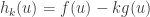$h_k(u) = f(u)-kg(u)$ for each $k \ge 0$ . The multiplier $k$ is then varied so that the constraint $g(u^*_k) = 0$ is satisfied.

Proving the Neyman-Pearson lemma

Now let’s use the method of undetermined multipliers to find most powerful tests. Recall the set $U$ which we are optimising over is the set of all tests $\phi$ . Recall also that we wish to optimise $f(\phi) = \mathbb{E}_1[\phi(X)]$ subject to the constraint $g(\phi) = \mathbb{E}_0[\phi(X)] - \alpha \le 0$ . The method of undetermined multipliers says that we should consider maximising the function

$h_k(\phi) = \mathbb{E}_1[\phi(X)] - k\mathbb{E}_0[\phi(X)]$ ,

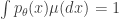
where $k \ge 0$ . Suppose that both $\mathbb{P}_0$ and $\mathbb{P}_1$ have densities₁ $p_0$ and $p_1$ with respect to some measure $\mu$ . We can we can write the above expectations as integrals. That is,

$\mathbb{E}_0[\phi(X)] = \int \phi(x)p_0(x)\mu(dx)$ and $\mathbb{E}_1[\phi(X)] = \int \phi(x)p_1(x)\mu(dx)$ .

Thus the function $h_k$ is equal to

$h_k(\phi) = \int \phi(x)p_1(x)\mu(dx)- k\int \phi(x)p_0(x)\mu(dx)=\int \phi(x)(p_1(x)-kp_0(x))\mu(dx)$ .

We now wish to maximise the function $h_k(\phi)$ . Recall that $\phi$ is a function that take values in $[0,1]$ . Thus, the integral

$\int \phi(x)(p_1(x)-kp_0(x))\mu(dx)$ ,

is maximised if and only if $\phi(x)=1$ when $p_1(x)-kp_0(x) > 0$ and $\phi(x)=0$ when $p_1(x)-kp_0(x) < 0$ . Note that $p_1(x)-kp_0(x) > 0$ if and only if $\frac{p_1(x)}{p_0(x)} > k$ . Thus for each $k \ge 0$ , a test $\phi_k$ maximises $h_k(\phi)$ if and only if

$\phi_k(x) = \begin{cases} 1 & \text{if } \frac{p_1(x)}{p_0(x)} > k,\\ 0 &\text{if } \frac{p_1(x)}{p_0(x)} < k. \end{cases}$

The method of undetermined multipliers says that if we can find $k$ so that the above is satisfied and $g(\phi_k) = 0$ , then $\phi_k$ is a most powerful test. Recall that $g(\phi_k)=0$ is equivalent to $\mathbb{E}_1[\phi(X)]=\alpha$ . By summarising the above argument, we arrive at the Neyman-Pearson lemma,

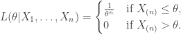
Neyman-Pearson Lemma₂: Suppose that $\phi$ is a test such that

$\mathbb{E}_0[\phi(X)] = \alpha$ , and
For some $k \ge 0$ , $\phi(x) = \begin{cases} 1 & \text{if } \frac{p_1(x)}{p_0(x)} > k,\\ 0 & \text{if } \frac{p_1(x)}{p_0(x)}< k.\end{cases}$

then $\phi$ is most powerful at level- $\alpha$ for testing $H_0 : X \sim \mathbb{P}_0$ against $H_1 : X \sim \mathbb{P}_1$ .

The magic of Neyman-Pearson

By learning about undetermined multipliers I’ve been able to better understand the proof of the Neyman-Pearson lemma. I now view it is as clever solution to a constrained optimisation problem rather than something that comes out of nowhere.

There is, however, a different aspect of Neyman-Pearson that continues to surprise me. This aspect is the usefulness of the lemma. At first glance the Neyman-Pearson lemma seems to be a very specialised result because it is about simple hypothesis testing. In reality most interesting hypothesis tests have composite nulls or composite alternatives or both. It turns out that Neyman-Pearson is still incredibly useful for composite testing. Through ideas like monotone likelihood ratios, least favourable distributions and unbiasedness, the Neyman-Pearson lemma or similar ideas can be used to find optimal tests in a variety of settings.

Thus I must admit that the title of this blog post is a little inaccurate and deceptive. I do believe that, given the tools of undetermined multipliers and the set up of simple hypothesis testing, one is naturally led to the Neyman-Pearson lemma. However, I don’t believe that many could have realised how useful and interesting simple hypothesis testing would be.

Footnotes

The assumption that $\mathbb{P}_0$ and $\mathbb{P}_1$ have densities with respect to a common measure $\mu$ is not a restrictive assumption since one can always take $\mu = \mathbb{P}_0+\mathbb{P}_1$ and the apply Radon-Nikodym. However there is often a more natural choice of $\mu$ such as Lebesgue measure on $\mathbb{R}^d$ or the counting measure on $\mathbb{N}$ .
What I call the Neyman-Pearson lemma is really only a third of the Neyman-Pearson lemma. There are two other parts. One that guarantees the existence of a most powerful test and one that is a partial converse to the statement in this post.

Leverages Scores

I am very excited to be writing a blog post again – it has been nearly a year! This post marks a new era for the blog. In September I started a statistics PhD at Stanford University. I am really enjoying my classes and I am learning a lot. I might have to change the name of the blog soon but for now let’s stick with “Maths to Share” although you will undoubtedly see more and more statistics here.

Today I would like to talk about leverages scores. Leverages scores are a way to quantify how sensitive a model is and they can be used to explain the different behaviour in these two animations

Linear Models

I recently learnt about leverage scores in the applied statistics course STATS 305A. This course is all about the linear model. In the linear model we assume with have $n$ data points $(x_i,y_i)$ where $x_i$ is a vector in $\mathbb{R}^d$ and $y_i$ is a number in $\mathbb{R}$ . We model $y_i$ as a linear function of $x_i$ plus noise. That is we assume $y_i = x_i^T\beta + \varepsilon_i$ , where $\beta \in \mathbb{R}^d$ is a unknown vector of coefficients and $\varepsilon_i$ is a random variable with mean $0$ and variance $\sigma^2$ . We also require that for $i \neq j$ , the random variable $\varepsilon_i$ is uncorrelated with $\varepsilon_j$ .

We can also write this as a matrix equation. Define $y$ to be the vector with entries $y_i$ and define $X$ to be the matrix with rows $x_i^T$ , that is

$y = \begin{bmatrix} y_1\\ y_2 \\ \vdots \\ y_n \end{bmatrix} \in \mathbb{R}^n$ and $X = \begin{bmatrix} -x_1^T-\\-x_2^T-\\ \vdots \\ -x_n^T-\end{bmatrix} \in \mathbb{R}^{n \times d}.$

Then our model can be rewritten as

$y = X\beta + \varepsilon,$

where $\varepsilon \in \mathbb{R}^n$ is a random vector with mean $0$ and covariance matrix $\sigma^2 I_n$ . To simplify calculations we will assume that $X$ contains an intercept term. This means that the first column of $X$ consists of all 1’s.

In the two animations at the start of this post we have two nearly identical data sets. The data sets are an example of simple regression when each vector $x_i$ is of the form $(1,z_i)$ where $z_i$ is a number. The values $z_i$ are on the horizontal axis and the values $y_i$ are on the vertical axis.

Estimating the coefficients

In the linear model we wish to estimate the parameter $\beta$ which contains the coefficients of our model. That is, given a sample $(y_i,x_i)_{i=1}^n$ , we wish to construct a vector $\widehat{\beta}$ which approximates the true parameter $\beta$ . In ordinary least square regression we choose $\widehat{\beta}$ to be the vector $b \in \mathbb{R}^d$ that minimizes the quantity

$\sum_{i=1}^n (x_i^T b - y_i)^2=\left \Vert Xb - y \right \Vert_2^2$ .

Differentiating with respect to $b$ and setting the derivative equal to $0$ shows that $\widehat{\beta}$ is a solution to the normal equations:

$X^TXb = X^T y.$

We will assume that the matrix $X^TX$ is invertible. In this case then the normal equations have a unique solution $\widehat{\beta} = (X^TX)^{-1}X^T y$ .

Now that we have our estimate $\widehat{\beta}$ , we can do prediction. If we are given a new value $x' \in \mathbb{R}^d$ we would use $x'^T\widehat{\beta}$ to predict the corresponding value of $y'$ . This was how the straight lines in the two animations were calculated.

We can also calculate the model’s predicted values for the data $x_i$ that we used to fit the model. These are denoted by $\widehat{y}$ . Note that

$\widehat{y} = X\widehat{\beta} = X(X^TX)^{-1}X^Ty = Hy,$

where $H = X(X^TX)^{-1}X^T$ is called the hat matrix for the model (since it puts the hat $\widehat{ }$ on $y$ .

Leverage scores

We are now ready to talk about leverage scores and the two animations. For reference, here they are again:

In both animations the stationary line corresponds to an estimator $\widehat{\beta}$ that was calculated using only the black data points. The red points are new data points with different $x$ values and varying $y$ values. The moving line corresponds to an estimator $\widehat{\beta}$ calculated using the red data point as well as all the black points. We can see immediately that if the red point is far away from the “bulk” of the other $x$ points, then the moving line is a lot more sensitive to the $y$ value of the red point.

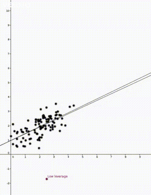
The leverage score of a data point $(x_i,y_i)$ is defined to be $\frac{\partial \widehat{y}_i}{\partial y_i}.$ That is, the leverage score tells us how much does the prediction $\widehat{y}_i$ change if we change $y_i$ .

Since $\widehat{y} = Hy$ , the leverage score of $(x_i,y_i)$ is $H_{ii}$ , the $i^{th}$ diagonal element of the hat matrix $H$ . The idea is that if a data point $(x_i,y_i)$ has a large leverage score, then the model is more sensitive to changes in that value of $y_i$ .

This can be seen in a leave one out calculation. This calculation tells us what we should expect if we make a leave-one-out model – a model that uses all the data points apart from one. In our animations, this corresponds to the stationary line.

The leave one out calculation says that the predicted value using all the data is always between the true value and the predicted value from the leave-one-out model. In our animations this can be seen by noting that the moving line (the full model) is always between the red point (the true value) and the stationary line (the leave-one-out model).

Furthermore the leverage score tells us exactly how close the predicted value is to the true value. We can see that the moving line is much closer to the red dot in the high leverage example on the right than the low leverage example on the left.

Mahalanobis distance

We now know that the two animations are showing the sensitivity of a model to two different data points. We know that a model is more sensitive to point with high leverage than to points with low leverage. We still haven’t spoken about why some point have higher leverage and why the point on the right has higher leverage.

It turns out that leverage score are measuring how far away a data point is from the “bulk” of the other $x_i$ ‘s. More specifically in a one dimensional example like what we have in the animations

$H_{ii} = \frac{1}{n}\left(\frac{1}{S^2}(x_i-\bar{x})^2+1\right),$

where $n$ is the number of data points, $\bar{x} = \frac{1}{n}\sum_{j=1}^n x_j$ is the sample mean and $S^2 = \frac{1}{n}\sum_{j=1}^n (x_j-\bar{x})^2$ is the sample variance. Thus high leverage scores correspond to points that are far away from the centre of our data $x_i$ . In higher dimensions a similar result holds if we measure distance using Mahalanobis distance.

The mean of the black data points is approximately 2 and so we can now see why the second point has higher leverage. The two animations were made in Geogebra. You can play around with them here and here.

[Link Post] Complexity Penalties in Statistical Machine Learning

Earlier in the year I wrote a post on Less Wrong about some of the material I learnt at the 2019 AMSI Summer School. You can read it here. On a related note, applications are open for the 2020 AMSI Summer School at La Trobe University. I highly recommend attending!