Probability – Maths to Share

Poisson approximations to the negative binomial distribution

This post is an introduction to the negative binomial distribution and a discussion of different ways of approximating the negative binomial distribution.

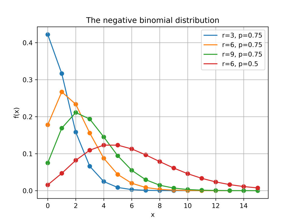
The negative binomial distribution describes the number of times a coin lands on tails before a certain number of heads are recorded. The distribution depends on two parameters $p$ and $r$ . The parameter $p$ is the probability that the coin lands on heads and $r$ is the number of heads. If $X$ has the negative binomial distribution, then $X = x$ means in the first $x+r-1$ tosses of the coin, there were $r-1$ heads and that toss number $x+r$ was a head. This means that the probability that $X=x$ is given by

$\displaystyle{f(x) = \binom{x+r-1}{r-1}p^{r}\left(1-p\right)^x}$

Here is a plot of the function $f(x)$ for different values of $r$ and $p$ .

Poisson approximations

When the parameter $r$ is large and $p$ is close to one, the negative binomial distribution can be approximated by a Poisson distribution. More formally, suppose that $r(1-p)=\lambda$ for some positive real number $\lambda$ . If $r$ is large then, the negative binomial random variable with parameters $p$ and $r$ , converges to a Poisson random variable with parameter $\lambda$ . This is illustrated in the picture below where three negative binomial distributions with $r(1-p)=5$ approach the Poisson distribution with $\lambda =5$ .

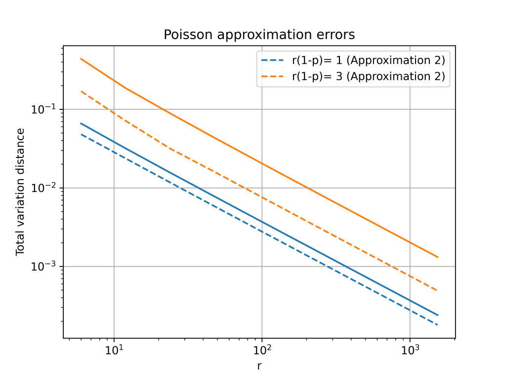
Total variation distance is a common way to measure the distance between two discrete probability distributions. The log-log plot below shows that the error from the Poisson approximation is on the order of $1/r$ and that the error is bigger if the limiting value of $r(1-p)$ is larger.

It turns out that is is possible to get a more accurate approximation by using a different Poisson distribution. In the first approximation, we used a Poisson random variable with mean $\lambda = r(1-p)$ . However, the mean of the negative binomial distribution is $r(1-p)/p$ . This suggests that we can get a better approximation by setting $\lambda = r(1-p)/p$ .

The change from $\lambda = r(1-p)$ to $\lambda = r(1-p)/p$ is a small because $p \approx 1$ . However, this small change gives a much better approximation, especially for larger values of $r(1-p)$ . The below plot shows that both approximations have errors on the order of $1/r$ , but the constant for the second approximation is much better.

Second order accurate approximation

It is possible to further improve the Poisson approximation by using a Gram–Charlier expansion. A Gram–Charlier approximation for the Poisson distribution is given in this paper.¹ The approximation is

$\displaystyle{f_{GC}(x) = P_\lambda(x) - \frac{1}{2}(1-p)\left((x-\lambda)P_\lambda(x)-(x-1-\lambda)P_\lambda(x-1)\right)},$

where $\lambda = \frac{k(1-p)}{p}$ as in the second Poisson approximation and $P_\lambda(x)$ is the Poisson pmf evaluated at $x$ .

The Gram–Charlier expansion is considerably more accurate than either Poisson approximation. The errors are on the order of $1/r^2$ . This higher accuracy means that the error curves for the Gram–Charlier expansion has a steeper slope.

The approximation is given in equation (4) of the paper and is stated in terms of the CDF instead of the PMF. The equation also contains a small typo, it should say $\frac{1}{2}q$ instead of $\frac{1]{2}p$ . ↩︎

The discrete arcsine distribution

The discrete arcsine distribution is a probability distribution on $\{0,1,\ldots,n\}$ . It is a u-shaped distribution. There are peaks at $0$ and $n$ and a dip in the middle. The figure below shows the probability distribution function for $n=10,15, 20$ .

The probability distribution function of the arcsine distribution is given by

$\displaystyle{p_n(k) = \frac{1}{2^{2n}}\binom{2k}{k}\binom{2n-2k)}{n-k}\text{ for } k \in \{0,1,\ldots,n\}}$

The discrete arcsine distribution is related to simple random walks and to an interesting Markov chain called the Burnside process. The connection with simple random walks is explained in Chapter 3, Volume 1 of An Introduction to Probability and its applications by William Feller. The connection to the Burnside process was discovered by Persi Diaconis in Analysis of a Bose-Einstein Markov Chain.

The discrete arcsine distribution gets its name from the continuous arcsine distribution. Suppose $X_n$ is distributed according to the discrete arcsine distribution with parameter $n$ . Then the normalized random variables $X_n/n$ converges in distribution to the continuous arcsine distribution on $[0,1]$ . The continuous arcsine distribution has the probability density function

$\displaystyle{f(x) = \frac{1}{\pi\sqrt{x(1-x)}} \text{ for } 0 \le x \le 1}$

This means that continuous arcsine distribution is a beta distribution with $\alpha=\beta=1/2$ . It is called the arcsine distribution because the cumulative distribution function involves the arcsine function

$\displaystyle{F(x) = \int_0^x f(y)dy = \frac{2}{\pi}\arcsin(\sqrt{x}) \text{ for } 0 \le x \le 1}$

There is another connection between the discrete and continuous arcsine distributions. The continuous arcsine distribution can be used to sample the discrete arcsine distribution. The two step procedure below produces a sample from the discrete arcsine distribution with parameter $n$ :

Sample $p$ from the continuous arcsine distribution.
Sample $X$ from the binomial distribution with parameters $n$ and $p$ .

This means that the discrete arcsine distribution is actually the beta-binomial distribution with parameters $\alpha = \beta =1/2$ . I was surprised when I was told this, and couldn’t find a reference. The rest of this blog post proves that the discrete arcsine distribution is an instance of the beta-binomial distribution.

As I showed in this post, the beta-binomial distribution has probability distribution function:

$\displaystyle{q_{\alpha,\beta,n}(k) = \binom{n}{k}\frac{B(k+\alpha, n-k+\alpha)}{B(a,b)}},$

where $B(x,y)=\frac{\Gamma(x)\Gamma(y)}{\Gamma(x+y)}$ is the Beta-function. To show that the discrete arc sine distribution is an instance of the beta-binomial distribution we need that $p_n(k)=q_{1/2,1/2,n}(k)$ . That is

$\displaystyle{ \binom{n}{k}\frac{B(k+1/2, n-k+1/2)}{B(1/2,1/2)} = \frac{1}{2^{2n}}\binom{2k}{k}\binom{2n-2k}{n-k}}$ ,

for all $k = 0,1,\ldots,n$ . To prove the above equation, we can first do some simplifying to $q_{1/2,1/2,n}(k)$ . By definition

$\displaystyle{\frac{B(k+1/2, n-k+1/2)}{B(1/2,1/2)} = \frac{\frac{\Gamma(k+1/2)\Gamma(n-k+1/2)}{\Gamma(n+1)}}{\frac{\Gamma(1/2)\Gamma(1/2)}{\Gamma(1)}} = \frac{1}{n!}\frac{\Gamma(k+1/2)}{\Gamma(1/2)}\frac{\Gamma(n-k+1/2)}{\Gamma(1/2)}}$ ,

where I have used that $\Gamma(m)=(m-1)!$ factorial if $m$ is a natural number. The Gamma function $\Gamma(x)$ also satisfies the property $\Gamma(x+1)=x\Gamma(x)$ . Using this repeatedly gives

$\displaystyle{\Gamma(k+1/2) = (k-1/2) \times (k-3/2) \times \cdots \times \frac{3}{2}\times\frac{1}{2}\times\Gamma(1/2) }.$

This means that

$\displaystyle{\frac{\Gamma(k+1/2)}{\Gamma(1/2)} = (k-1/2) \times (k-3/2) \times \cdots \times \frac{3}{2}\times\frac{1}{2} = \frac{(2k-1)\times(2k-3)\times \cdots \times 3 \times 1}{2^k}=\frac{(2k-1)!!}{2^k}},$

where $(2k-1)!!=(2k-1)\times (2k-3)\times\cdots \times 3 \times 1$ is the double factorial. The same reasoning gives

$\displaystyle{\frac{\Gamma(n-k+1/2)}{\Gamma(1/2)} =\frac{(2n-2k-1)!!}{2^{n-k}}}.$

And so

$\displaystyle{q_{1/2,1/2,n}(k) =\frac{1}{2^nk!(n-k)!}(2k-1)!!(2n-2k-1)!!}.$

We’ll now show that $p_n(k)$ is also equal to the above final expression. Recall

$\displaystyle{p_n(k) = \frac{1}{2^{2n}} \binom{2k}{k}\binom{2(n-k)}{n-k} = \frac{1}{2^{2n}}\frac{(2k)!(2(n-k))!}{k!k!(n-k)!(n-k)!} = \frac{1}{2^nk!(n-k)!}\frac{(2k)!}{k!2^k}\frac{(2n-2k)!}{(n-k)!2^{n-k}}}.$

And so it suffices to show $\frac{(2k)!}{k!2^k} = (2k-1)!!$ (and hence $\frac{(2n-2k)!}{(n-k)!2^{n-k}}=(2n-2k-1)!!$ ). To see why this last claim holds, note that

$\displaystyle{\frac{(2k)!}{k!2^k} = \frac{(2k)\times (2k-1)\times(2k-2)\times\cdots\times 3 \times 2 \times 1}{(2k)\times (2k-2)\times \cdots \times 2} = (2k-1)!!}$

Showing that $p_{n}(k)=q_{n,1/2,1/2}(k)$ as claimed.

The sample size required for importance sampling

My last post was about using importance sampling to estimate the volume of high-dimensional ball. The two figures below compare plain Monte Carlo to using importance sampling with a Gaussian proposal. Both plots use $M=1,000$ samples to estimate $v_n$ , the volume of an $n$ -dimensional ball

A friend of mine pointed out that the relative error does not seem to increase with the dimension $n$ . He thought it was too good to be true. It turns out he was right and the relative error does increase with dimension but it increases very slowly. To estimate $v_n$ the number of samples needs to grow on the order of $\sqrt{n}$ .

To prove this, we will use the paper The sample size required for importance sampling by Chatterjee and Diaconis [1]. This paper shows that the sample size for importance sampling is determined by the Kullback-Liebler divergence. The relevant result from their paper is Theorem 1.3. This theorem is about the relative error in using importance sampling to estimate a probability.

In our setting the proposal distribution is $Q=\mathcal{N}(0,\frac{1}{n}I_n)$ . That is the distribution $Q$ is an $n$ -dimensional Gaussian vector with mean $0$ and covariance $\frac{1}{n}I_n$ . The conditional target distribution is $P$ the uniform distribution on the $n$ dimensional ball. Theorem 1.3 in [1] tells us how many samples are needed to estimate $v_n$ . Informally, the required sample size is $M = O(\exp(D(P \Vert Q)))$ . Here $D(P\Vert Q)$ is the Kullback-Liebler divergence between $P$ and $Q$ .

To use this theorem we need to compute $D(P \Vert Q)$ . Kullback-Liebler divergence is defined as integral. Specifically

$\displaystyle{D(P\Vert Q) = \int_{\mathbb{R}^n} \log\frac{P(x)}{Q(x)}P(x)dx}$

Computing the high-dimensional integral above looks challenging. Fortunately, it can reduced to a one-dimensional integral. This is because both the distributions $P$ and $Q$ are rotationally symmetric. To use this, define $P_r,Q_r$ to be the distribution of the norm squared under $P$ and $Q$ . That is if $X \sim P$ , then $\Vert X \Vert_2^2 \sim P_R$ and likewise for $Q_R$ . By the rotational symmetry of $P$ and $Q$ we have

$D(P\Vert Q) = D(P_R \Vert Q_R).$

We can work out both $P_R$ and $Q_R$ . The distribution $P$ is the uniform distribution on the $n$ -dimensional ball. And so for $X \sim P$ and any $r \in [0,1]$

$\mathbb{P}(\Vert X \Vert_2^2 \le r) = \frac{v_n r^n}{v_n} = r^n.$

Which implies that $P_R$ has density $P_R(r)=nr^{n-1}$ . This means that $P_R$ is a Beta distribution with parameters $\alpha = n, \beta = 1$ . The distribution $Q$ is a multivariate Gaussian distribution with mean $0$ and variance $\frac{1}{n}I_n$ . This means that if $X \sim Q$ , then $\Vert X \Vert_2^2 = \sum_{i=1}^n X_i^2$ is a scaled chi-squared variable. The shape parameter of $Q_R$ is $n$ and scale parameter is $1/n$ . The density for $Q_R$ is therefor

$Q_R(r) = \frac{n^{n/2}}{2^{n/2}\Gamma(n/2)}r^{n/2-1}e^{-nx/2}$

The Kullback-Leibler divergence between $P$ and $Q$ is therefor

$\displaystyle{D(P\Vert Q)=D(P_R\Vert Q_R) = \int_0^1 \log \frac{P_R(r)}{Q_R(r)} P_R(r)dr}$

Getting Mathematica to do the above integral gives

$D(P \Vert Q) = -\frac{1+2n}{2+2n} + \frac{n}{2}\log(2 e) - (1-\frac{n}{2})\log n + \log \Gamma(\frac{n}{2}).$

Using the approximation $\log \Gamma(z) \approx (z-\frac{1}{2})\log(z)-z+O(1)$ we get that for large $n$

$D(P \Vert Q) = \frac{1}{2}\log n + O(1)$ .

And so the required number of samples is $O(\exp(D(P \Vert Q)) = O(\sqrt{n}).$

[1] Chatterjee, Sourav, and Persi Diaconis. “THE SAMPLE SIZE REQUIRED IN IMPORTANCE SAMPLING.” The Annals of Applied Probability 28, no. 2 (2018): 1099–1135. https://www.jstor.org/stable/26542331. (Public preprint here https://arxiv.org/abs/1511.01437)

The beta-binomial distribution

The beta-binomial model is a Bayesian model used to analyze rates. For a great derivation and explanation of this model, I highly recommend watching the second lecture from Richard McElreath’s course Statistical Rethinking. In this model, the data, $X$ , is assumed to be binomially distributed with a fixed number of trail $N$ but an unknown rate $\rho \in [0,1]$ . The rate $\rho$ is given a $\text{Beta}(a,b)$ prior. That is the prior distribution of $\rho$ has a density

$p(\rho) = \frac{1}{B(a,b)} \rho^{a-1}(1-\rho)^{b-1},$

where $B(a,b) =\int_0^1 \rho^{a-1}(1-\rho)^{b-1}d\rho$ is a normalizing constant. The model can thus be written as

$\rho \sim \text{Beta}(a,b),$
$X | \rho \sim \text{Binom}(N,\rho).$

This is a conjugate model, meaning that the posterior distribution of $\rho$ is again a beta distribution. This can be seen by using Bayes rule

$p(\rho | X) \propto p(X| \rho)p(\rho) \propto \rho^X(1-\rho)^{N-X}\rho^{a-1}(1-\rho)^{b-1}=\rho^{X+a-1}(1-\rho)^{(N-X)+b-1}.$

The last expression is proportional to a beta density., specifically $\rho | X \sim \text{Beta}(X+a, N-X+b)$ .

The marginal distribution of $X$

In the above model we are given the distribution of $\rho$ and the conditional distribution of $X|\rho$ . To calculate the distribution of $X$ , we thus need to marginalize over $\rho$ . Specifically,

$\displaystyle{p(X) = \int_0^1 p(X,\rho)d\rho = \int_0^1 p(X| \rho)p(\rho)d\rho.}$

The term inside the above integral is

$\displaystyle{p(X| \rho)p(\rho) = \binom{N}{X}\rho^X(1-\rho)^{N-X}\frac{1}{B(a,b)}\rho^{a-1}(1-\rho)^{b-1} = \frac{\binom{N}{X}}{B(a,b)}\rho^{X+a-1}(1-\rho)^{N-X+b-1} }.$

Thus,

$\displaystyle{p(X) = \frac{\binom{N}{X}}{B(a,b)} \int_0^1 \rho^{X+a-1}(1-\rho)^{N-X+b-1}d\rho = \binom{N}{X}\frac{B(X+a, N-X+a)}{B(a,b)}}.$

This distribution is called the beta-binomial distribution. Below is an image from Wikipedia showing a graph of $p(X)$ for $N=10$ and a number of different values of $a$ and $b$ . You can see that, especially for small value of $a$ and $b$ the distribution is a lot more spread out than the binomial distribution. This is because there is randomness coming from both $\rho$ and the binomial conditional distribution.

A plot of the beta-binomial distribution for different values of the parameters a and b. For small values of a and b, the distribution is very spread out.