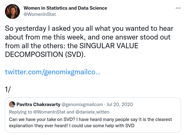
The singular value decomposition (SVD) is a powerful matrix decomposition. It is used all the time in statistics and numerical linear algebra. The SVD is at the heart of the principal component analysis, it demonstrates what’s going on in ridge regression and it is one way to construct the Moore-Penrose inverse of a matrix. For more SVD love, see the tweets below.
In this post I’ll define the SVD and prove that it always exists. At the end we’ll look at some pictures to better understand what’s going on.
Definition
Let  be a
be a  matrix. We will define the singular value decomposition first in the case
  . The SVD consists of three matrix
  and
and  such that
  . The matrix
  is required to be diagonal with non-negative diagonal entries
  . These numbers are called the singular values of . The matrices
  and
and  are required to orthogonal matrices so that
  , the
, the  identity matrix. Note that since is square we also have
  however we won’t have
  unless
  .
.
In the case when  , we can define the SVD of in terms of the SVD of
  . Let
. Let  and
and  be the SVD of so that
  . The SVD of is then given by transposing both sides of this equation giving
  and
and  .
.
Construction
The SVD of a matrix can be found by iteratively solving an optimisation problem. We will first describe an iterative procedure that produces matrices and . We will then verify that  and satisfy the defining properties of the SVD.
We will construct the matrices and one column at a time and we will construct the diagonal matrix one entry at a time. To construct the first columns and entries, recall that the matrix is really a linear function from  to
to  given by
  . We can thus define the operator norm of via

where  represents the Euclidean norm of
  and
and  is the Euclidean norm of
  . The set of vectors
  is a compact set and the function
  is continuous. Thus, the supremum used to define
  is achieved at some vector
  . Define
  . If
. If  , then define
  . If
. If  , then define
  to be an arbitrary vector in with
  . To summarise we have
We have now started to fill in our SVD. The number  is the first singular value of and the vectors
  and will be the first columns of the matrices and respectively.
Now suppose that we have found the first  singular values
  and the first columns of and . If
  , then we are done. Otherwise we repeat a similar process.
Let  and
and  be the first columns of and . The vectors split into two subspaces. These subspaces are
  and
and  , the orthogonal compliment of
  . By restricting to
  we get a new linear map
  . Like before, the operator norm of
  is defined to be
 .
.
Since  we must have

The set  is a compact set and thus there exists a vector
  such that
  . As before define
  and
and  if
if  . If
. If  , then define
  to be any vector in
  that is orthogonal to
  .
.
This process repeats until eventually and we have produced matrices and . In the next section, we will argue that these three matrices satisfy the properties of the SVD.
Correctness
The defining properties of the SVD were given at the start of this post. We will see that most of the properties follow immediately from the construction but one of them requires a bit more analysis. Let ![U = [u_1,\ldots,u_p]](https://s0.wp.com/latex.php?latex=U+%3D+%5Bu_1%2C%5Cldots%2Cu_p%5D&bg=ffffff&fg=333333&s=0&c=20201002) ,
,  and
and ![V= [v_1,\ldots,v_p]](https://s0.wp.com/latex.php?latex=V%3D+%5Bv_1%2C%5Cldots%2Cv_p%5D&bg=ffffff&fg=333333&s=0&c=20201002) be the output from the above construction.
be the output from the above construction.
First note that by construction  are orthogonal since we always had
  . It follows that the matrix is orthogonal and so
 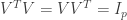 .
.
The matrix is diagonal by construction. Furthermore, we have that  for every . This is because both
  and
and  were defined as maximum value of over different subsets of . The subset for contained the subset for and thus
  .
.
We’ll next verify that . Since is orthogonal, the vectors  form an orthonormal basis for . It thus suffices to check that
 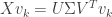 for
for  . Again by the orthogonality of we have that
  , the
, the  standard basis vector. Thus,

Above, we used that was a diagonal matrix and that  is the column of . If
  , then
  by definition. If
  , then
  and so
 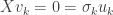 also. Thus, in either case,
 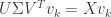 and so
  .
.
The last property we need to verify is that is orthogonal. Note that this isn’t obvious. At each stage of the process, we made sure that . However, in the case that  , we simply defined . It is not clear why this would imply that is orthogonal to .
It turns out that a geometric argument is needed to show this. The idea is that if was not orthogonal to  for some
  , then
  couldn’t have been the value that maximises .
Let  and be two columns of with
  and
and  . We wish to show that
  . To show this we will use the fact that and
  are orthonormal and perform “polar-interpolation“. That is, for
 ![\lambda \in [0,1]](https://s0.wp.com/latex.php?latex=%5Clambda+%5Cin+%5B0%2C1%5D&bg=ffffff&fg=333333&s=0&c=20201002) , define
, define

Since  and are orthogonal, we have that

Furthermore  is orthogonal to
  . Thus, by definition of ,

By the linearity of and the definitions of  ,
,
 .
.
Since  and
and  , we have

Rearranging and dividing by  gives,
 for all
 ![\lambda \in (0,1]](https://s0.wp.com/latex.php?latex=%5Clambda+%5Cin+%280%2C1%5D&bg=ffffff&fg=333333&s=0&c=20201002)
Taking  gives
gives  . Performing the same polar interpolation with
  shows that
  and hence .
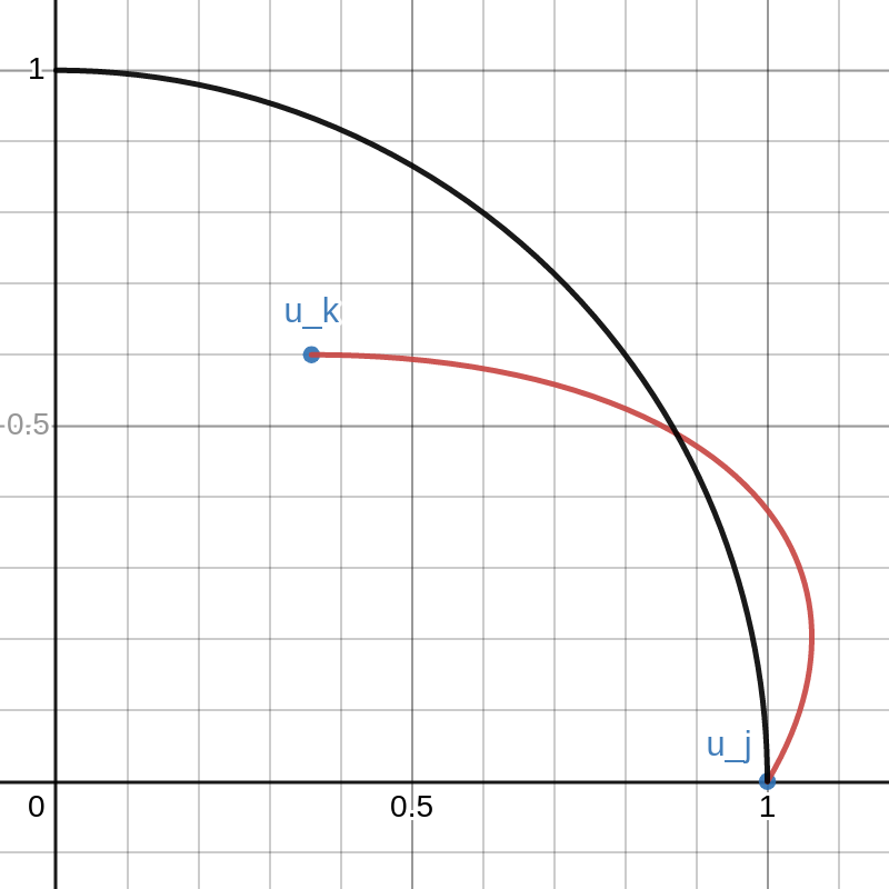
We have thus proved that is orthogonal. This proof is pretty “slick” but it isn’t very illuminating. To better demonstrate the concept, I made an interactive Desmos graph that you can access here.
This graph shows example vectors  . The vector is fixed at
  and a quarter circle of radius
  is drawn. Any vectors
  that are outside this circle have
  .
.
The vector can be moved around inside this quarter circle. This can be done either cby licking and dragging on the point or changing that values of  and
and  on the left. The red curve is the path of
 .
.
As  goes from
  to , the path travels from to .
Note that there is a portion of the red curve near that is outside the black circle. This corresponds to a small value of  that results in
  contradicting the definition of . By moving the point around in the plot you can see that this always happens unless lies exactly on the y-axis. That is, unless is orthogonal to .


, any matrix
of size
that satisfy the above condition.


 -algebra generated by the collection. In my post I give an example which shows that you need the collection to be closed under finite intersections. I also show that you need to have at least four points in the space to find such an example.
 .
.  be a normally distributed random vector with mean
  . Given a vector
  , the non-central chi-squared distribution with
  is the distribution of the quantity
 . As this notation suggests, the distribution of
  depends only on
  , the norm of
  . The first few times I heard this fact, I had no idea why it would be true (and even found it a little
  such that
  . We wish to show that if
  , then
  .
. have the same norm there exists an orthogonal matrix
  such that
  . Since
  . Furthermore, since
  . This is because, for all
  ,
,
 .
. have the same distribution, we can conclude that
  has the same distribution as
  . Since
  , we are done.
 depends only on the norm of the vector
  and then return
  . But for large values of
  where
where  is the vector with a
 follows the regular chi-squared distribution with
  degrees of freedom and is independent of
  . The regular chi-squared distribution is a special case of the gamma distribution and can be effectively sampled with rejection sampling for large shape parameter (see
  , so for large values of
  . Finally to get a sample from
  .
. 
 .
. .
. with
with  and
and  .
.
 is a one-dimensional exponential family written in canonical form. That is,
  and there exists a reference measure
  has a density
  with respect to
 is a sufficient statistic for the model
  . The function
  is the log-partition function for the family
  implies that

 . Thus,
![A'(\theta) = \mathbb{E}_\theta[T(X)]](https://s0.wp.com/latex.php?latex=A%27%28%5Ctheta%29+%3D+%5Cmathbb%7BE%7D_%5Ctheta%5BT%28X%29%5D&bg=ffffff&fg=333333&s=0&c=20201002) , the expectation of
, the expectation of  and we want to use this sample to estimate
  . One way to estimate
 .
.
 solves the equation,
![A'(\widehat{\theta}) = \mathbb{E}_{\widehat{\theta}}[T(X)]](https://s0.wp.com/latex.php?latex=A%27%28%5Cwidehat%7B%5Ctheta%7D%29+%3D+%5Cmathbb%7BE%7D_%7B%5Cwidehat%7B%5Ctheta%7D%7D%5BT%28X%29%5D&bg=ffffff&fg=333333&s=0&c=20201002) . Thus the MLE is the solution to the equation,
. Thus the MLE is the solution to the equation,![\mathbb{E}_{\widehat{\theta}}[T(X)] = \frac{1}{n}\sum_{i=1}^n T(X_i)](https://s0.wp.com/latex.php?latex=%5Cmathbb%7BE%7D_%7B%5Cwidehat%7B%5Ctheta%7D%7D%5BT%28X%29%5D+%3D+%5Cfrac%7B1%7D%7Bn%7D%5Csum_%7Bi%3D1%7D%5En+T%28X_i%29&bg=ffffff&fg=333333&s=0&c=20201002) .
. where
where ![[0,\theta]](https://s0.wp.com/latex.php?latex=%5B0%2C%5Ctheta%5D&bg=ffffff&fg=333333&s=0&c=20201002) . A minimal sufficient statistic for this model is
. A minimal sufficient statistic for this model is  – the maximum of
  . Given what we saw before, we might imague that the MLE for this model would be a method of moments estimator for
  is,
is,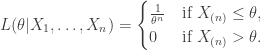
 . However, under
  has a
has a  distribution. Thus,
 ![\mathbb{E}_\theta[X_{(n)}] = \theta \frac{n}{n+1}](https://s0.wp.com/latex.php?latex=%5Cmathbb%7BE%7D_%5Ctheta%5BX_%7B%28n%29%7D%5D++%3D+++%5Ctheta+%5Cfrac%7Bn%7D%7Bn%2B1%7D&bg=ffffff&fg=333333&s=0&c=20201002) so the method of moments estimator would be
so the method of moments estimator would be 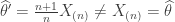 .
. in my book when the proof was finished. Later in class we learnt the method of undetermined multipliers and suddenly I saw where the Neyman-Pearson lemma came from.
  which is a realisation of some random variable
  or from the distribution
  . Thus, our null hypothesis is
  and our alternative hypothesis is
  .
. against
  is a function
  that takes in data
 ![\phi(x) \in [0,1]](https://s0.wp.com/latex.php?latex=%5Cphi%28x%29+%5Cin+%5B0%2C1%5D&bg=ffffff&fg=333333&s=0&c=20201002) . The value
. The value  is the probability under the test
  , we always reject
  we never reject
  , we reject
  .
. ![\mathbb{E}_0[\phi(X)]](https://s0.wp.com/latex.php?latex=%5Cmathbb%7BE%7D_0%5B%5Cphi%28X%29%5D&bg=ffffff&fg=333333&s=0&c=20201002) and
and ![\mathbb{E}_1[\phi(X)]](https://s0.wp.com/latex.php?latex=%5Cmathbb%7BE%7D_1%5B%5Cphi%28X%29%5D&bg=ffffff&fg=333333&s=0&c=20201002) be the expectation of
be the expectation of  under
under  is a number between
 ![\mathbb{E}_1[\phi(X)] \le \alpha](https://s0.wp.com/latex.php?latex=%5Cmathbb%7BE%7D_1%5B%5Cphi%28X%29%5D+%5Cle+%5Calpha&bg=ffffff&fg=333333&s=0&c=20201002) . A test
. A test  , the test
 ![\mathbb{E}_1[\phi'(X)] \le \mathbb{E}_1[\phi(X)]](https://s0.wp.com/latex.php?latex=%5Cmathbb%7BE%7D_1%5B%5Cphi%27%28X%29%5D+%5Cle+%5Cmathbb%7BE%7D_1%5B%5Cphi%28X%29%5D&bg=ffffff&fg=333333&s=0&c=20201002) .
.![\mathbb{E}_0[\phi(X)] \le \alpha](https://s0.wp.com/latex.php?latex=%5Cmathbb%7BE%7D_0%5B%5Cphi%28X%29%5D+%5Cle+%5Calpha&bg=ffffff&fg=333333&s=0&c=20201002)
 and we wish to maximise
  subject to the constraint
  .
.  is given by
 ![f(\phi) = \mathbb{E}_1[\phi(X)]](https://s0.wp.com/latex.php?latex=f%28%5Cphi%29+%3D+%5Cmathbb%7BE%7D_1%5B%5Cphi%28X%29%5D&bg=ffffff&fg=333333&s=0&c=20201002) . That is,
. That is,  is the power of the test
  is given by
 ![g(\phi)=\mathbb{E}_1[\phi(X)]-\alpha](https://s0.wp.com/latex.php?latex=g%28%5Cphi%29%3D%5Cmathbb%7BE%7D_1%5B%5Cphi%28X%29%5D-%5Calpha&bg=ffffff&fg=333333&s=0&c=20201002) so that
so that  if and only if
  is such that:
  ,
, , such that
  maximises
  over all
  .
. . By assumption we know that
  and
and  .
. and so
  and so
  as needed.
  that maximise
  for each
  is satisfied.
![g(\phi) = \mathbb{E}_0[\phi(X)] - \alpha \le 0](https://s0.wp.com/latex.php?latex=g%28%5Cphi%29+%3D+%5Cmathbb%7BE%7D_0%5B%5Cphi%28X%29%5D+-+%5Calpha+%5Cle+0&bg=ffffff&fg=333333&s=0&c=20201002) . The method of undetermined multipliers says that we should consider maximising the function
. The method of undetermined multipliers says that we should consider maximising the function ![h_k(\phi) = \mathbb{E}_1[\phi(X)] - k\mathbb{E}_0[\phi(X)]](https://s0.wp.com/latex.php?latex=h_k%28%5Cphi%29+%3D+%5Cmathbb%7BE%7D_1%5B%5Cphi%28X%29%5D+-+k%5Cmathbb%7BE%7D_0%5B%5Cphi%28X%29%5D&bg=ffffff&fg=333333&s=0&c=20201002) ,
, and
and  with respect to some measure
 ![\mathbb{E}_0[\phi(X)] = \int \phi(x)p_0(x)\mu(dx)](https://s0.wp.com/latex.php?latex=%5Cmathbb%7BE%7D_0%5B%5Cphi%28X%29%5D+%3D+%5Cint+%5Cphi%28x%29p_0%28x%29%5Cmu%28dx%29&bg=ffffff&fg=333333&s=0&c=20201002) and
and ![\mathbb{E}_1[\phi(X)] = \int \phi(x)p_1(x)\mu(dx)](https://s0.wp.com/latex.php?latex=%5Cmathbb%7BE%7D_1%5B%5Cphi%28X%29%5D+%3D+%5Cint+%5Cphi%28x%29p_1%28x%29%5Cmu%28dx%29&bg=ffffff&fg=333333&s=0&c=20201002) .
.  is equal to
 .
. . Recall that
 ![[0,1]](https://s0.wp.com/latex.php?latex=%5B0%2C1%5D&bg=ffffff&fg=333333&s=0&c=20201002) . Thus, the integral
. Thus, the integral ,
, when
when  and
and  . Note that
  . Thus for each
  maximises
 , then
  is equivalent to
 ![\mathbb{E}_1[\phi(X)]=\alpha](https://s0.wp.com/latex.php?latex=%5Cmathbb%7BE%7D_1%5B%5Cphi%28X%29%5D%3D%5Calpha&bg=ffffff&fg=333333&s=0&c=20201002) . By summarising the above argument, we arrive at the Neyman-Pearson lemma,
. By summarising the above argument, we arrive at the Neyman-Pearson lemma,![\mathbb{E}_0[\phi(X)] = \alpha](https://s0.wp.com/latex.php?latex=%5Cmathbb%7BE%7D_0%5B%5Cphi%28X%29%5D+%3D+%5Calpha&bg=ffffff&fg=333333&s=0&c=20201002) , and
, and
 and the apply Radon-Nikodym. However there is often a more natural choice of
  or the counting measure on
  .
.

 where
where  is a vector in
  is a number in
  . We model
  , where
  is a unknown vector of coefficients and
  is a random variable with mean
  . We also require that for
  , the random variable
  .
.  to be the vector with entries
  , that is
  and
and 

 is a random vector with mean
  . To simplify calculations we will assume that
  where
where  is a number. The values
  , we wish to construct a vector
  which approximates the true parameter
  that minimizes the quantity
  .
.
 is invertible. In this case then the normal equations have a unique solution
  .
.  we would use
  to predict the corresponding value of
  . This was how the straight lines in the two animations were calculated.
  . Note that
 is called the hat matrix for the model (since it puts the hat
  on
on 

 That is, the leverage score tells us how much does the prediction
  change if we change
  , the leverage score of
  , the
, the  diagonal element of the hat matrix
  . The idea is that if a data point
 is the sample mean and
  is the sample variance. Thus high leverage scores correspond to points that are far away from the centre of our data