Monte Carlo integration in high dimensions

Monte Carlo integration

John Cook recently wrote a cautionary blog post about using Monte Carlo to estimate the volume of a high-dimensional ball. He points out that if $\mathbf{X}=(X_1,\ldots,X_n)$ are independent and uniformly distributed on the interval $[-1,1]$ then

$\displaystyle{\mathbb{P}(X_1^2 + X_2^2 + \cdots + X_n^2 \le 1) = \frac{v_n}{2^n}},$

where $v_n$ is the volume of an $n$ -dimensional ball with radius one. This observation means that we can use Monte Carlo to estimate $v_n$ .

To do this we repeatedly sample vectors $\mathbf{X}_m = (X_{m,1},\ldots,X_{m,n})$ with $X_{m,i}$ uniform on $[-1,1]$ and $m$ ranging from $1$ to $M$ . Next, we count the proportion of vectors $\mathbf{X}_m$ with $X_{1,m}^2 + \cdots + X_{n,m}^2 \le 1$ . Specifically, if $Z_m$ is equal to one when $X_{1,m}^2 + \cdots + X_{n,m}^2 \le 1$ and equal to zero otherwise, then by the law of large numbers

$\displaystyle{\frac{1}{M}\sum_{m=1}^M Z_m \approx \frac{v_n}{2^n}}$

Which implies

$v_n \approx 2^n \frac{1}{M}\sum_{m=1}^M Z_m$

This method of approximating a volume or integral by sampling and counting is called Monte Carlo integration and is a powerful general tool in scientific computing.

The problem with Monte Carlo integration

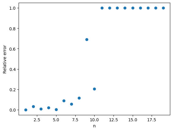
As pointed out by John, Monte Carlo integration does not work very well in this example. The plot below shows a large difference between the true value of $v_n$ with $n$ ranging from $1$ to $20$ and the Monte Carlo approximation with $M = 1,000$ .

The problem is that $v_n$ is very small and the probability $v_n/2^n$ is even smaller! For example when $n = 10$ , $v_n/2^n \approx 0.0025$ . This means that in our one thousand samples we only expect two or three occurrences of the event $X_{m,1}^2 + \cdots + X_{m,n}^2 \le 1$ . As a result our estimate has a high variance.

The results get even worse as $n$ increases. The probability $v_n/2^n$ does to zero faster than exponentially. Even with a large value of $M$ , our estimate will be zero. Since $v_n \neq 0$ , the relative error in the approximation is 100%.

Importance sampling

Monte Carlo can still be used to approximate $v_n$ . Instead of using plain Monte Carlo, we can use a variance reduction technique called importance sampling (IS). Instead of sampling the points $X_{m,1},\ldots, X_{m,n}$ from the uniform distribution on $[-1,1]$ , we can instead sample the from some other distribution called a proposal distribution. The proposal distribution should be chosen so that that the event $X_{m,1}^2 +\cdots +X_{m,n}^2 \le 1$ becomes more likely.

In importance sampling, we need to correct for the fact that we are using a new distribution instead of the uniform distribution. Instead of the counting the number of times $X_{m,1}^2+\cdots+X_{m,n}^2 \le 1$ , we give weights to each of samples and then add up the weights.

If $p$ is the density of the uniform distribution on $[-1,1]$ (the target distribution) and $q$ is the density of the proposal distribution, then the IS Monte Carlo estimate of $v_n$ is

$\displaystyle{\frac{1}{M}\sum_{m=1}^M Z_m \prod_{i=1}^n \frac{p(X_{m,i})}{q(X_{m,i})}},$

where as before $Z_m$ is one if $X_{m,1}^2+\cdots +X_{m,n}^2 \le 1$ and $Z_m$ is zero otherwise. As long as $q(x)=0$ implies $p(x)=0$ , the IS Monte Carlo estimate will be an unbiased estimate of $v_n$ . More importantly, a good choice of the proposal distribution $q$ can drastically reduce the variance of the IS estimate compared to the plain Monte Carlo estimate.

In this example, a good choice of proposal distribution is the normal distribution with mean $0$ and variance $1/n$ . Under this proposal distribution, the expected value of $X_{m,1}^2 +\cdots+ X_{m,n}^2$ is one and so the event $X_{m,1}^2 + \cdots + X_{m,n}^2 \le 1$ is much more likely.

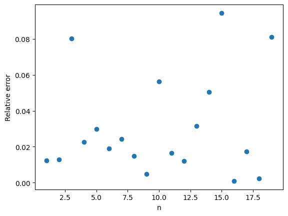
Here are the IS Monte Carlo estimates with again $M = 1,000$ and $n$ ranging from $1$ to $20$ . The results speak for themselves.

The relative error is typically less than 10%. A big improvement over the 100% relative error of plain Monte Carlo.

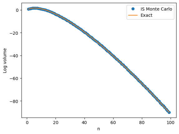
The next plot shows a close agreement between $v_n$ and the IS Monte Carlo approximation on the log scale with $n$ going all the way up to $100$ .

Notes

There are exact formulas for $v_n$ (available on Wikipedia). I used these to compare the approximations and compute relative errors. There are related problems where no formulas exist and Monte Carlo integration is one of the only ways to get an approximate answer.
The post by John Cook also talks about why the central limit theorem can’t be used to approximate $v_n$ . I initially thought a technique called large deviations could be used to approximate $v_n$ but again this does not directly apply. I was happy to discover that importance sampling worked so well!

Monte Carlo integration in high dimensions