This post is an introduction to the negative binomial distribution and a discussion of different ways of approximating the negative binomial distribution.
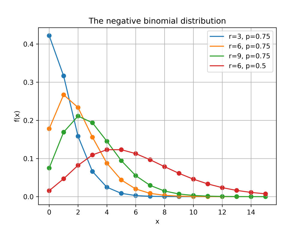
The negative binomial distribution describes the number of times a coin lands on tails before a certain number of heads are recorded. The distribution depends on two parameters 


Here is a plot of the function 
Poisson approximations
When the parameter 


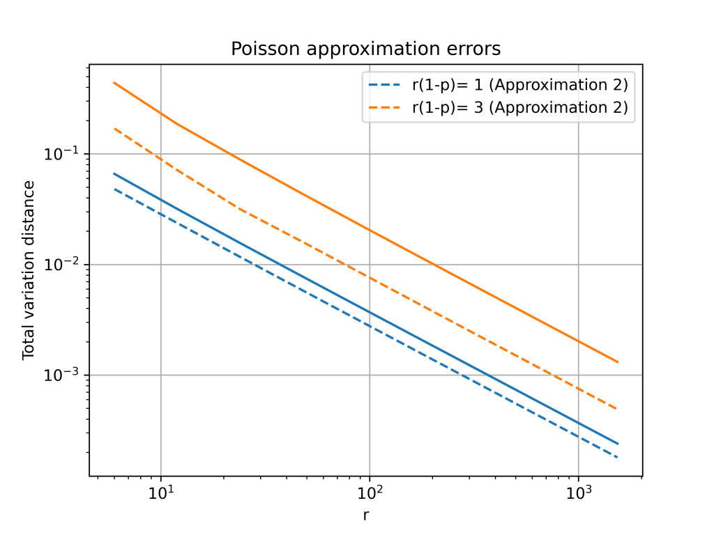
Total variation distance is a common way to measure the distance between two discrete probability distributions. The log-log plot below shows that the error from the Poisson approximation is on the order of 


It turns out that is is possible to get a more accurate approximation by using a different Poisson distribution. In the first approximation, we used a Poisson random variable with mean 


The change from 
Second order accurate approximation
It is possible to further improve the Poisson approximation by using a Gram–Charlier expansion. A Gram–Charlier approximation for the Poisson distribution is given in this paper.1 The approximation is

where 


The Gram–Charlier expansion is considerably more accurate than either Poisson approximation. The errors are on the order of 

- The approximation is given in equation (4) of the paper and is stated in terms of the CDF instead of the PMF. The equation also contains a small typo, it should say
instead of
. ↩︎


 balls draw without replacement from an urn with
  white balls and
  black balls. The probability of having
 possible ways to sample
  black balls in total. Of these possibilities, there are
  ways of selecting exactly
  colours instead of
  . Suppose that the urn contains
  balls of the first colour,
  balls of the second colour and so on. The total number of balls in the urn is
  . Next we draw
  be the number of balls of colour
  in our sample. The vector
  follows the multivariate hypergeometric distribution. The vector
  and
and  . The probability of observing
 possible ways of sampling
  balls in total. Likewise, The number of ways of choosing
  balls of colour
  is
is  .
. without replacement. The numbers
  represent the numbers with colour 1, and let
  represent the numbers with colour 2 and so on. Suppose that
  is the sample of size
 will be distributed according to the multivariate hypergeometric distribution. This method of sampling has complexity on the order of
  . This is because sampling a random number of size
  and we need to sample
  we can treat the balls of colour
  as “white” and all the other colours as “black”. This means that marginally,
  and
and  and
and  . Furthermore, conditional on
  , is also hypergeometric. The parameters for
  ,
,  and
and  . In fact, all of the conditionals of
  . The overall complexity of the sequential method is therefore on the order of
  which can be much smaller than
  be i.i.d. geometric random variables with success probability
  . Next, define
  . I wanted to know the limiting distribution of
  as
as  and
and  . I was particularly interested in the case when
  .
. as
as 

 and has fluctuations of order
  . Furthermore, these fluctuations are distributed according to the
  .
. converge to exponential random variables. Exponential random variables are nicer to work because they have a continuous distribution.
  where
where  are exponentially distributed. Next, we will derive the main result for the exponential random variables. Then, in the next section, we will prove that
  where
where  ,
,  . The condition
  is equivalent to
  for all
  . Since the
 . Since
 . We want to show that it holds for
  converges in distribution to an exponential random variable. This is a result that holds for a single random variable. For an approximation like
  , we need a result that works for every
 . This is because
 ![\mathbb{P}(X_i \le x) = 1-(1-p)^{[x]}](https://s0.wp.com/latex.php?latex=%5Cmathbb%7BP%7D%28X_i+%5Cle+x%29+%3D+1-%281-p%29%5E%7B%5Bx%5D%7D&bg=ffffff&fg=333333&s=0&c=20201002) and
and  . This means that

 we will get
 and
and  . This means that the random variable
  has the same limit as
  also has the same limit as
  . Since
  and
and 
![U \in [-1,1]](https://s0.wp.com/latex.php?latex=U+%5Cin+%5B-1%2C1%5D&bg=ffffff&fg=333333&s=0&c=20201002) and
and ![V \in [0,1]](https://s0.wp.com/latex.php?latex=V+%5Cin+%5B0%2C1%5D&bg=ffffff&fg=333333&s=0&c=20201002) are independent and uniformly distributed. Then
are independent and uniformly distributed. Then  has the ratio of uniforms distribution. The plot below shows a histogram based on 10,000 samples from the ratio of uniforms distribution
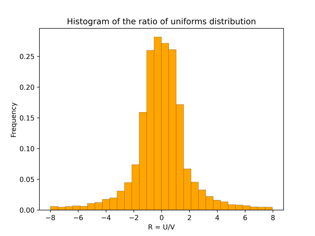
 also has a table mountain shape.


 corresponds to the flat part of the table mountain. The second case corresponds to the sloping curves. The rest of this post use geometry to derive the above formula for
  .
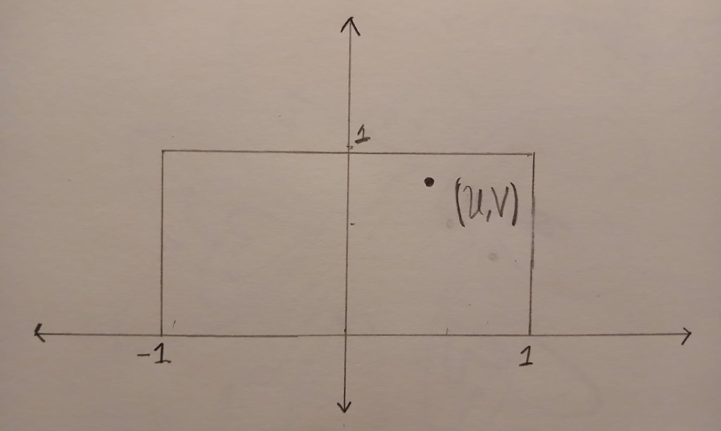
. is uniformly distributed in the box
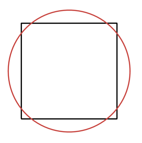
 ![B=[-1,1] \times [0,1]](https://s0.wp.com/latex.php?latex=B%3D%5B-1%2C1%5D+%5Ctimes+%5B0%2C1%5D&bg=ffffff&fg=333333&s=0&c=20201002) . The image below shows an example of a point
. The image below shows an example of a point  .
.
 and goes through
  . The
. The  .
.
![[R,R+dR]](https://s0.wp.com/latex.php?latex=%5BR%2CR%2BdR%5D&bg=ffffff&fg=333333&s=0&c=20201002) is
is ![\displaystyle{\frac{\text{Area}(\{(u,v) \in B : u/v \in [R, R+dR]\})}{\text{Area}(B)} = \frac{1}{2}\text{Area}(\{(u,v) \in B : u/v \in [R, R+dR]\}).}](https://s0.wp.com/latex.php?latex=%5Cdisplaystyle%7B%5Cfrac%7B%5Ctext%7BArea%7D%28%5C%7B%28u%2Cv%29+%5Cin+B+%3A+u%2Fv+%5Cin+%5BR%2C+R%2BdR%5D%5C%7D%29%7D%7B%5Ctext%7BArea%7D%28B%29%7D+%3D+%5Cfrac%7B1%7D%7B2%7D%5Ctext%7BArea%7D%28%5C%7B%28u%2Cv%29+%5Cin+B+%3A+u%2Fv+%5Cin+%5BR%2C+R%2BdR%5D%5C%7D%29.%7D&bg=ffffff&fg=333333&s=0&c=20201002)
![\displaystyle{h(R) = \lim_{dR \to 0} \frac{1}{2dR}\text{Area}(\{(u,v) \in B : u/v \in [R, R+dR]\})}.](https://s0.wp.com/latex.php?latex=%5Cdisplaystyle%7Bh%28R%29+%3D+%5Clim_%7BdR+%5Cto+0%7D+%5Cfrac%7B1%7D%7B2dR%7D%5Ctext%7BArea%7D%28%5C%7B%28u%2Cv%29+%5Cin+B+%3A+u%2Fv+%5Cin+%5BR%2C+R%2BdR%5D%5C%7D%29%7D.&bg=ffffff&fg=333333&s=0&c=20201002)
 and
and ![\{(u,v) \in B : u/v \in [R, R+dR]\}](https://s0.wp.com/latex.php?latex=%5C%7B%28u%2Cv%29+%5Cin+B+%3A+u%2Fv+%5Cin+%5BR%2C+R%2BdR%5D%5C%7D&bg=ffffff&fg=333333&s=0&c=20201002) is a triangle. This triangle is drawn in blue below.
is a triangle. This triangle is drawn in blue below.
 . The perpendicular height of the triangle from the horizontal edge is
 ![\displaystyle{\text{Area}(\{(u,v) \in B : u/v \in [R, R+dR]\}) =\frac{1}{2}\times dR \times 1=\frac{dR}{2}}.](https://s0.wp.com/latex.php?latex=%5Cdisplaystyle%7B%5Ctext%7BArea%7D%28%5C%7B%28u%2Cv%29+%5Cin+B+%3A+u%2Fv+%5Cin+%5BR%2C+R%2BdR%5D%5C%7D%29+%3D%5Cfrac%7B1%7D%7B2%7D%5Ctimes+dR+%5Ctimes+1%3D%5Cfrac%7BdR%7D%7B2%7D%7D.&bg=ffffff&fg=333333&s=0&c=20201002)
![R \in [-1,1]](https://s0.wp.com/latex.php?latex=R+%5Cin+%5B-1%2C1%5D&bg=ffffff&fg=333333&s=0&c=20201002) we have
we have

 . The perpendicular height of the triangle from the vertical edge is
 ![\displaystyle{\text{Area}(\{(u,v) \in B : u/v \in [R, R+dR]\}) =\frac{1}{2}\times \frac{dR}{R(R+dR)} \times 1=\frac{dR}{2R(R+dR)}}.](https://s0.wp.com/latex.php?latex=%5Cdisplaystyle%7B%5Ctext%7BArea%7D%28%5C%7B%28u%2Cv%29+%5Cin+B+%3A+u%2Fv+%5Cin+%5BR%2C+R%2BdR%5D%5C%7D%29+%3D%5Cfrac%7B1%7D%7B2%7D%5Ctimes+%5Cfrac%7BdR%7D%7BR%28R%2BdR%29%7D+%5Ctimes+1%3D%5Cfrac%7BdR%7D%7B2R%28R%2BdR%29%7D%7D.&bg=ffffff&fg=333333&s=0&c=20201002)

 and
and  . This is because the ratio of uniform distribution has heavy tails. This meant that there were some very large values of
  . It is a u-shaped distribution. There are peaks at
  .
.

 is distributed according to the discrete arcsine distribution with parameter
  converges in distribution to the continuous arcsine distribution on
 ![[0,1]](https://s0.wp.com/latex.php?latex=%5B0%2C1%5D&bg=ffffff&fg=333333&s=0&c=20201002) . The continuous arcsine distribution has the probability density function
. The continuous arcsine distribution has the probability density function
 . It is called the arcsine distribution because the cumulative distribution function involves the arcsine function
 . I was surprised when I was told this, and couldn’t find a reference. The rest of this blog post proves that the discrete arcsine distribution is an instance of the beta-binomial distribution.
 is the Beta-function. To show that the discrete arc sine distribution is an instance of the beta-binomial distribution we need that
  . That is
 ,
, . To prove the above equation, we can first do some simplifying to
  . By definition
 ,
, factorial if
  is a natural number. The Gamma function
  also satisfies the property
  . Using this repeatedly gives

 is the double factorial. The same reasoning gives

 is also equal to the above final expression. Recall
 (and hence
  ). To see why this last claim holds, note that
 as claimed.
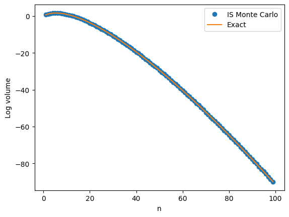
 samples to estimate
  , the volume of an

 .
. . That is the distribution
  is an
is an  . The conditional target distribution is
  the uniform distribution on the
  . Here
  is the Kullback-Liebler divergence between
  . Kullback-Liebler divergence is defined as integral. Specifically
 to be the distribution of the norm squared under
  , then
  and likewise for
  . By the rotational symmetry of
 and
and ![r \in [0,1]](https://s0.wp.com/latex.php?latex=r+%5Cin+%5B0%2C1%5D&bg=ffffff&fg=333333&s=0&c=20201002)

 . This means that
  . The distribution
  , then
  is a scaled chi-squared variable. The shape parameter of


 we get that for large
  .
.
 are independent and uniformly distributed on the interval
 ![[-1,1]](https://s0.wp.com/latex.php?latex=%5B-1%2C1%5D&bg=ffffff&fg=333333&s=0&c=20201002) then
then
 with
with  uniform on
  with
with  . Specifically, if
  is equal to one when

 and the Monte Carlo approximation with
  .
. is even smaller! For example when
  ,
,  . This means that in our one thousand samples we only expect two or three occurrences of the event
  . As a result our estimate has a high variance.
 , the relative error in the approximation is 100%.
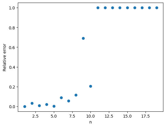
 from the uniform distribution on
  becomes more likely.
 , we give weights to each of samples and then add up the weights.
  is the density of the proposal distribution, then the IS Monte Carlo estimate of
 and
and  implies
  , the IS Monte Carlo estimate will be an unbiased estimate of
  is one and so the event
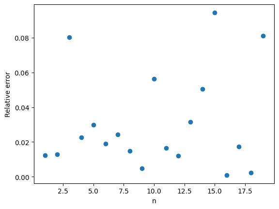
 .
.
 matrix
  is orthogonal if
  . The set of all
  . The uniform distribution on
  is an independent standard normal random variable. Let
  be the columns of
  be the result of applying Gram-Schmidt to
  . Then the matrix
 ![M=[q_1,q_2,\ldots,q_n] \in O_n](https://s0.wp.com/latex.php?latex=M%3D%5Bq_1%2Cq_2%2C%5Cldots%2Cq_n%5D+%5Cin+O_n&bg=ffffff&fg=333333&s=0&c=20201002) is distributed according to Haar measure.
is distributed according to Haar measure. is a QR-factorization of
  is distributed according to Haar measure. However, most numerical libraries do not use Gram-Schmidt to calculate the QR-factorization of a matrix. This means that if you generate a random
 , the top-left entry of a matrix
  . We then compute a diagonal matrix
  with
with  . Then, the matrix
  is Haar distributed. The following python code thus samples a Haar distributed matrix in