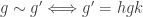
Like my previous post, this blog is also motivated by a comment by Professor Persi Diaconis in his recent Stanford probability seminar. The seminar was about a way of “collapsing” a random walk on a group to a random walk on the set of double cosets. In this post, I’ll first define double cosets and then go over the example Professor Diaconis used to make us probabilists and statisticians more comfortable with all the group theory he was discussing.
Double cosets
Let be a group and let and be two subgroups of . For each , the -double coset containing is defined to be the set
To simplify notation, we will simply write double coset instead of -double coset. The double coset of can also be defined as the equivalence class of under the relation
for some and
Like regular cosets, the above relation is indeed an equivalence relation. Thus, the group can be written as a disjoint union of double cosets. The set of all double cosets of is denoted by . That is,
Note that if we take , the trivial subgroup, then the double cosets are simply the left cosets of , . Likewise if , then the double cosets are the right cosets of , . Thus, double cosets generalise both left and right cosets.
Double cosets in
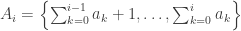
Fix a natural number . A partition of is a finite sequence such that , and . For each partition of , , we can form a subgroup of the symmetric group . The subgroup contains all permutations such that fixes the sets . Meaning that for all . Thus, a permutation must individually permute the elements of , the elements of and so on. This means that, in a natural way,
If we have two partitions and , then we can form two subgroups and and consider the double cosets . The claim made in the seminar was that the double cosets are in one-to-one correspondence with contingency tables with row sums equal to and column sums equal to . Before we explain this correspondence and properly define contingency tables, let’s first consider the cases when either or is the trivial subgroup.
Left cosets in
Note that if , then is the trivial subgroup and, as noted above, is simply equal to . We will see that the cosets in can be described by forgetting something about the permutations in .
We can think of the permutations in as all the ways of drawing without replacement balls labelled . We can think of the partition as a colouring of the balls by colours. We colour balls by the first colour , then we colour the second colour and so on until we colour the final colour . Below is an example when is equal to 6 and .
The first three balls are coloured green, the next two are coloured red and the last ball is coloured blue.
Note that a permutation is in if and only if we draw the balls by colour groups, i.e. we first draw all the balls with colour , then we draw all the balls with colour and so on. Thus, continuing with the previous example, the permutation below is in but is not in .
The permutation is in because the colours are in their original order but is not in because the colours are rearranged.
It turns out that we can think of the cosets in as what happens when we “forget” the labels and only remember the colours of the balls. By “forgetting” the labels we mean only paying attention to the list of colours. That is for all , if and only if the list of colours from the draw is the same as the list of colours from the draw . Thus, the below two permutations define the same coset of
When we forget the labels and only remember the colours, the permutations and look the same and thus are in the same left coset of .
To see why this is true, note that if and only if for some . Furthermore, if and only if maps each colour group to itself. Recall that function composition is read right to left. Thus, the equation means that if we first relabel the balls according to and then draw the balls according to , then we get the result as just drawing by . That is, for some if and only if drawing by is the same as first relabelling the balls within each colour group and then drawing the balls according to . Thus, , if and only if when we forget the labels of the balls and only look at the colours, and give the same list of colours. This is illustrated with our running example below.
If we permute the balls according to and the draw according to , then the resulting draw is the same as if we had not permuted and drawn according to . That is, .
Right cosets of
Typically, the subgroup is not a normal subgroup of . This means that the right coset will not equal the left coset . Thus, colouring the balls and forgetting the labelling won’t describe the right cosets . We’ll see that a different type of forgetting can be used to describe .
Fix a partition and now, instead of considering colours, think of different people . As before, a permutation can be thought of drawing balls labelled without replacement. We can imagine giving the first balls drawn to person , then giving the next balls to the person and so on until we give the last balls to person . An example with and is drawn below.
Person receives the ball labelled by 6 followed by the ball labelled 3, person receives ball 2 and then ball 1 and finally person receives ball 4 followed by ball 5.
Note that if and only if person receives the balls with labels in any order. Thus, in the below example but .
When the balls are drawn according to , person receives the balls with labels and , and thus . On the other hand, if the balls are drawn according to , the people receive different balls and thus .
It turns out the cosets are exactly determined by “forgetting” the order in which each person received their balls and only remembering which balls they received. Thus, the two permutation below belong to the same coset in .
When we forget the order in which each person receive their balls, the permutations and become the same and thus . Note that if we coloured the balls according to the permutation , then we could see that .
To see why this is true in general, consider two permutations . The permutations result in each person receiving the same balls if and only if after we can apply a permutation that fixes each subset and get . That is, and result in each person receiving the same balls if and only if for some . Thus, are the same after forgetting the order in which each person received their balls if and only if . This is illustrated below,
If we first draw the balls according to and then permute the balls according to , then the resulting draw is the same as if we had drawn according to and not permuted afterwards. That is, .
We can thus see why . A left coset correspond to pre-composing with elements of and a right cosets correspond to post-composing with elements of .
Contingency tables
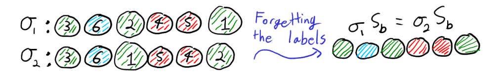
With the last two sections under our belts, describing the double cosets is straight forward. We simply have to combine our two types of forgetting. That is, we first colour the balls with colours according to . We then draw the balls without replace and give the balls to different people according . We then forget both the original labels and the order in which each person received their balls. That is, we only remember the number of balls of each colour each person receives. Describing the double cosets by “double forgetting” is illustrated below with and .
The permutations and both result in person receiving one green ball and one blue ball. The two permutations also results in and both receiving one green ball and one red ball. Thus, and are both in the same -double coset. Note however that and .
The proof that double forgetting does indeed describe the double cosets is simply a combination of the two arguments given above. After double forgetting, the number of balls given to each person can be recorded in an table. The entry of the table is simply the number of balls person receives of colour . Two permutations are the same after double forgetting if and only if they produce the same table. For example, and above both produce the following table
Green ()
Red ()
Blue ()
Total
Person
1
0
1
2
Person
1
1
0
2
Person
1
1
0
2
Total
3
2
1
6
By the definition of how the balls are coloured and distributed to each person we must have for all and
and
An table with entries satisfying the above conditions is called a contingency table. Given such a contingency table with entries where the rows sum to and the columns sum to , there always exists at least one permutation such that is the number of balls received by person of colour . We have already seen that two permutations produce the same table if and only if they are in the same double coset. Thus, the double cosets are in one-to-one correspondence with such contingency tables.
The hypergeometric distribution
I would like to end this blog post with a little bit of probability and relate the contingency tables above to the hyper geometric distribution. If for some , then the contingency tables described above have two rows and are determined by the values in the first row. The numbers are the number of balls of colour the first person receives. Since the balls are drawn without replacement, this means that if we put the uniform distribution on , then the vector follows the multivariate hypergeometric distribution. Thus, if we have a random walk on that quickly converges to the uniform distribution on , then we could use the double cosets to get a random walk that converges to the multivariate hypergeometric distribution (although there are smarter ways to do such sampling).
Something very exciting this afternoon. Professor Persi Diaconis was presenting at the Stanford probability seminar and the field with one element made an appearance. The talk was about joint work with Mackenzie Simper and Arun Ram. They had developed a way of “collapsing” a random walk on a group to a random walk on the set of double cosets. As an illustrative example, Persi discussed a random walk on given by multiplication by a random transvection (a map of the form , where ).
The Bruhat decomposition can be used to match double cosets of with elements of the symmetric group . So by collapsing the random walk on we get a random walk on for all prime powers . As Professor Diaconis said, you can’t stop him from taking and asking what the resulting random walk on is. The answer? Multiplication by a random transposition. As pointed sets are vector spaces over the field with one element and the symmetric groups are the matrix groups, this all fits with what’s expected of the field with one element.
This was just one small part of a very enjoyable seminar. There was plenty of group theory, probability, some general theory and engaging examples.
Update: I have written another post about some of the group theory from the seminar! You can read it here: Double cosets and contingency tables.
This post is about using ABC Radio’s API to create a record of all the songs played on Triple J in a given time period. An API (application programming interface) is a connection between two computer programs. Many websites have API’s that allow users to access data from that website. ABC Radio has an API that lets users access a record of the songs played on the station Triple J since around May 2014. Below I’ll show how to access this information and how to transform it into a format that’s easier to work with. All code can be found on GitHub here.
Packages
To access the API in R I used the packages “httr” and “jsonlite”. To transform the data from the API I used the packages “tidyverse” and “lubridate”.
If you type this into a web browser, you can see a bunch of text which actually lists information about the ten most recently played songs on ABC’s different radio stations. To see only the songs played on Triple J, you can go to:
shows information about the songs played in the 30 minutes after midnight UTC on the 16th of January last year. The last parameter that we will use is limit which specifies the number of songs to include. The link:
includes information about the most recently played song. The default for limit is 10 and the largest possible value is 100. We’ll see later that this cut off at 100 makes downloading a lot of songs a little tricky. But first let’s see how we can access the information from ABC Radio’s API in R.
Accessing an API in R
We now know how to use ABC Radio’s API to get information about the songs played on Triple J but how do we use this information in R and how is the information stored. The function GET from the package “httr” enables us to access the API in R. The input to GET is simply the same sort of URL that we’ve been using to view the API online. The below code stores information about the 5 songs played on Triple J just before 5 am on the 5th of May 2015
The line “Status: 200” tells us that we have successfully grabbed some data from the API. There are many other status codes that mean different thing but for now we’ll be happy remembering that “Status: 200” means everything has worked.
The information from the API is stored within the object res. To change it from a JSON file to a list we can use the function “fromJSON” from the library jsonlite. This is done below
data <- fromJSON(rawToChar(res$content))
names(data)
# "total"  "offset" "items"
The information about the individual songs is stored under items. There is a lot of information about each song including song length, copyright information and a link to an image of the album cover. For now, we’ll just try to find the name of the song, the name of the artist and the time the song played. We can find each of these under “items”. Finding the song title and the played time are pretty straight forward:
data$items$recording$title
# "First Light" "Dog"         "Begin Again" "Rot"         "Back To You"
data$items$played_time
# "2015-05-05T04:55:56+00:00" "2015-05-05T04:52:21+00:00" "2015-05-05T04:47:52+00:00" "2015-05-05T04:41:00+00:00" "2015-05-05T04:38:36+00:00"
Finding the artist name is a bit trickier.
data$items$recording$artists
# [[1]]
# entity       arid          name artwork
# 1 Artist maQeOWJQe1 Django Django    NULL
# links
# 1 Link, mlD5AM2R5J, http://musicbrainz.org/artist/4bfce038-b1a0-4bc4-abe1-b679ab900f03, 4bfce038-b1a0-4bc4-abe1-b679ab900f03, MusicBrainz artist, NA, NA, NA, service, musicbrainz, TRUE
# is_australian    type role
# 1            NA primary   NA
#
# [[2]]
# entity       arid      name artwork
# 1 Artist maXE59XXz7 Andy Bull    NULL
# links
# 1 Link, mlByoXMP5L, http://musicbrainz.org/artist/3a837db9-0602-4957-8340-05ae82bc39ef, 3a837db9-0602-4957-8340-05ae82bc39ef, MusicBrainz artist, NA, NA, NA, service, musicbrainz, TRUE
# is_australian    type role
# 1            NA primary   NA
# ....
# ....
We can see that each song actually has a lot of information about each artist but we’re only interested in the artist name. By using “map_chr()” from the library “tidyverse” we can grab each song’s artist name.
Using name[1] means that if there are multiple artists, then we only select the first one. With all of these in place we can create a tibble with the information about these five songs.
list <- data$items
tb <- tibble(
     song_title = list$recording$title,
     artist = map_chr(list$recording$artists, ~.$name[1]),
     played_time = ymd_hms(list$played_time)
) %>%
  arrange(played_time)
tb
# # A tibble: 5 x 3
# song_title  artist        played_time
# <chr>       <chr>         <dttm>
# 1 Back To You Twerps        2015-05-05 04:38:36
# 2 Rot         Northlane     2015-05-05 04:41:00
# 3 Begin Again Purity Ring   2015-05-05 04:47:52
# 4 Dog         Andy Bull     2015-05-05 04:52:21
# 5 First Light Django Django 2015-05-05 04:55:56
Downloading lots of songs
The maximum number of songs we can access from the API at one time is 100. This means that if we want to download a lot of songs we’ll need to use some sort of loop. Below is some code which takes in two dates and times in UTC and fetches all the songs played between the two times. The idea is simply to grab all the songs played in a five hour interval and then move on to the next five hour interval. I found including an optional value “progress” useful for the debugging. This code is from the file get_songs.r on my GitHub.
download <- function(from, to){
  base <- "https://music.abcradio.net.au/api/v1/plays/search.json?limit=100&offset=0&page=0&station=triplej&from="
  from_char <- format(from, "%Y-%m-%dT%H:%M:%S.000Z")
  to_char <- format(to, "%Y-%m-%dT%H:%M:%S.000Z")
  url <- paste0(base,
                from_char,
                "&to=",
                to_char)
  res <- GET(url)
  if (res$status == 200) {
    data <- fromJSON(rawToChar(res$content))
    list <- data$items
    tb <- tibble(
      song_title = list$recording$title,
      artist = map_chr(list$recording$artists, ~.$name[1]),
      played_time = ymd_hms(list$played_time)
    ) %>%
      arrange(played_time)
    return(tb)
  }
}

get_songs <- function(start, end, progress = FALSE){
  from <- ymd_hms(start)
  to <- from + dhours(5)
  end <- ymd_hms(end)

  songs <- NULL

  while (to < end) {
    if (progress) {
      print(from)
      print(to)
    }
    tb <- download(from, to)
    songs <- bind_rows(songs, tb)
    from <- to + dseconds(1)
    to <- to + dhours(5)
  }
  tb <- download(from, end)
  songs <- bind_rows(songs, tb)
  return(songs)
}
An example
Using the functions defined above, we can download all the sounds played in the year 2021 (measured in AEDT).
This code takes a little while to run so I have saved the output as a .csv file. There are lots of things I hope to do with this data such as looking at the popularity of different songs over time. For example, here’s a plot showing the cumulative plays of Genesis Owusu’s top six songs.
I’ve also looked at using the data from last year to get a list of Triple J’s most played artists. Unfortunately, it doesn’t line up with the official list. The issue is that I’m only recording the primary artist on each song and not any of the secondary artists. Hopefully I’ll address this in a later blog post! I would also like to an analysis of how plays on Triple J correlate with song ranking in the Hottest 100.
Maximum likelihood and the method of moments are two ways to estimate parameters from data. In general, the two methods can differ but for one-dimensional exponential families they produce the same estimates.
Suppose that is a one-dimensional exponential family written in canonical form. That is, and there exists a reference measure such each distribution has a density with respect to and,
The random variable is a sufficient statistic for the model . The function is the log-partition function for the family . The condition, implies that
It turns out that the function is differentiable and that differentiation and integration are exchangeable. This implies that
Note that . Thus,
This means that , the expectation of under .
Now suppose that we have an i.i.d. sample and we want to use this sample to estimate . One way to estimate is by maximum likelihood. That is, we choose the value of that maximises the likelihood,
When using the maximum likelihood estimator, it is often easier to work with the log-likelihood. The log-likelihood is,
.
Maximising the likelihood is equivalent to maximising the log-likelihood. For exponential families, the log-likelihood is a concave function of . Thus the maximisers can be found be differentiation and solving the first order equations. Note that,
Thus the maximum likelihood estimate (MLE) solves the equation,
But recall that . Thus the MLE is the solution to the equation,
.
Thus the MLE is the value of for which the expectation of matches the empirical average from our sample. That is, the maximum likelihood estimator for an exponential family is a method of moments estimator. Specifically, the maximum likelihood estimator matches the moments of the sufficient statistic .
A counter example
It is a special property of maximum likelihood estimators that the MLE is a method of moments estimator for the sufficient statistic. When we leave the nice world of exponential families, the estimators may differ.
Suppose that we have data where is the uniform distribution on . A minimal sufficient statistic for this model is – the maximum of . Given what we saw before, we might imague that the MLE for this model would be a method of moments estimator for but this isn’t the case.
The likelihood for is,
Thus the MLE is . However, under , has a distribution. Thus, so the method of moments estimator would be .
It is winter 2022 and my PhD cohort has moved on the second quarter of our first year statistics courses. This means we’ll be learning about generalised linear models in our applied course, asymptotic statistics in our theory course and conditional expectations and martingales in our probability course.
In the first week of our probability course we’ve been busy defining and proving the existence of the conditional expectation. Our approach has been similar to how we constructed the Lebesgue integral in the previous course. Last quarter, we first defined the Lebesgue integral for simple functions, then we used a limiting argument to define the Lebesgue integral for non-negative functions and then finally we defined the Lebesgue integral for arbitrary functions by considering their positive and negative parts.
Our approach to the conditional expectation has been similar but the journey has been different. We again started with simple random variables, then progressed to non-negative random variables and then proved the existence of the conditional expectation of any arbitrary integrable random variable. Unlike the Lebesgue integral, the hardest step was proving the existence of the conditional expectation of a simple random variable. Progressing from simple random variables to arbitrary random variables was a straight forward application of the monotone convergence theorem and linearity of expectation. But to prove the existence of the conditional expectation of a simple random variable we needed to work with projections in the Hilbert space .
Unlike the Lebesgue integral, defining the conditional expectation of a simple random variable is not straight forward. One reason for this is that the conditional expectation of a random variable need not be a simple random variable. This comment was made off hand by our Professor and sparked my curiosity. The following example is what I came up with. Below I first go over some definitions and then we dive into the example.
A simple random variable with a conditional expectation that is not simple
Let be a probability space and let be a sub--algebra. The conditional expectation of an integrable random variable is a random variable that satisfies the following two conditions:
The random variable is -measurable.
For all , , where is the indicator function of .
The conditional expectation of an integrable random variable is unique and always exists. One can think of as the expected value of given the information in .
A simple random variable is a random variable that take only finitely many values. Simple random variables are always integrable and so always exists but we will see that need not be simple.
Consider a random vector uniformly distributed on the square . Let be the unit disc . The random variable is a simple random variable since equals if and equals otherwise. Let the -algebra generated by . It turns out that
.
Thus is not a simple random variable. Let . Since is a continuous function of , the random variable is -measurable. Thus satisfies condition 1. Furthermore if , then for some measurable set . Thus equals if and only if and . Since is uniformly distributed we thus have
.
The random variable is uniformly distributed on and thus has density . Therefore,
.
Thus and therefore equals . Intuitively we can see this because given , we know that is when and that is otherwise. Since is uniformly distributed on the probability that is in is . Thus given , the expected value of is .
An extension
The previous example suggests an extension that shows just how “complicated” the conditional expectation of a simple random variable can be. I’ll state the extension as an exercise:
Let be any continuous function with . With and as above show that there exists a measurable set such that .
Last year sports climbing made its Olympic debut. My partner Claire is an avid climber and we watched some of the competition together. The method of ranking the competitors had some surprising consequences which are the subject of this blog.
In the finals, the climbers had to compete in three disciplines – speed climbing, bouldering and lead climbing. Each climber was given a rank for each discipline. For speed climbing, the rank was given based on how quickly the climbers scaled a set route. For bouldering and lead climbing, the rank was based on how far they climbed on routes none of them had seen before.
To get a final score, the ranks from the three disciplines are multiplied together. The best climber is the one with the lowest final score. For example, if a climber was 5th in speed climbing, 2nd in bouldering and 3rd in lead climbing, then they would have a final score of . A climber who came 8th in speed, 1st in bouldering and 2nd in lead climbing would have a lower (and thus better) final score of .
One thing that makes this scoring system interesting is that your final score is very dependent on how well your competitors perform. This was most evident during Jakob Schubert’s lead climb in the men’s final.
Lead climbing is the final discipline and Schubert was the last climber. This meant that ranks for speed climbing and bouldering were already decided. However, the final rankings of the climbers fluctuated hugely as Schubert scaled the 15 metre lead wall. This was because if a climber had done really well in the boulder and speed rounds, being overtaken by Schubert didn’t increase their final score by that much. However, if a climber did poorly in the previous rounds, then being overtaken by Schubert meant their score increased by a lot and they plummeted down the rankings. This can be visualised in the following plot:
Along the x-axis we have how far up the lead wall Schubert climbed (measured by the “hold” he had reached). On the y-axis we have the finalists’ ranking at different stages of Schubert’s climb. We can see that as Schubert climbed and overtook the other climbers the whole ranking fluctuated. Here is a similar plot which also shows when Schubert overtook each competitor on the lead wall:
The volatility of the rankings can really be seen by following Adam Ondra’s ranking (in purple). When Schubert started his climb, Ondra was ranked second. After Schubert passed Albert Gines Lopez, Ondra was ranked first. But then Schubert passed Ondra, Ondra finished the event in 6th place and Gines Lopez came first. If you go to the 4 hour and 27 minutes mark here you can watch Schubert’s climb and hear the commentator explain how both Gines Lopez and Ondra are in the running to win gold.
Similar things happened in the women’s finals. Janja Garnbret was the last lead climber in the women’s final. Here is the same plot which shows the climbers’ final rankings and lead ranking.
Garnbret was a favourite at the Olympics and had come fifth in the speed climbing and first in bouldering. This meant that as long as she didn’t come last in the lead climbing she would at least take home silver and otherwise she’ll get the gold. Garnbret ended up coming first in the lead climbing and we can see that as she overtook the last few climbers, their ranking fluctuated wildly.
Here is one more plot which shows each competitor’s final score at different points of Garnbret’s climb.
In the plot you can really see that, depending on how they performed in the previous two events, each climber’s score changed by a different amount once they were overtaken. It also shows how Garnbret is just so ahead of the competition – especially when you compare the men’s and women’s finals. Here is the same plot for the men. You can see that the men’s final scores were a lot closer together.
Before I end this post, I would like to make one comment about the culture of sport climbing. In this post I wanted to highlight how tumultuous and complicated the sport climbing rankings were but if you watched the athletes you’d have no idea the stakes were so high. The climbers celebrate their personal bests as if no one was watching, they trade ideas on how to tackle the lead wall and the day after the final, they returned to the bouldering wall to try the routes together. Sports climbing is such a friendly and welcoming sport and I would hate for my analysis to give anyone the wrong idea.
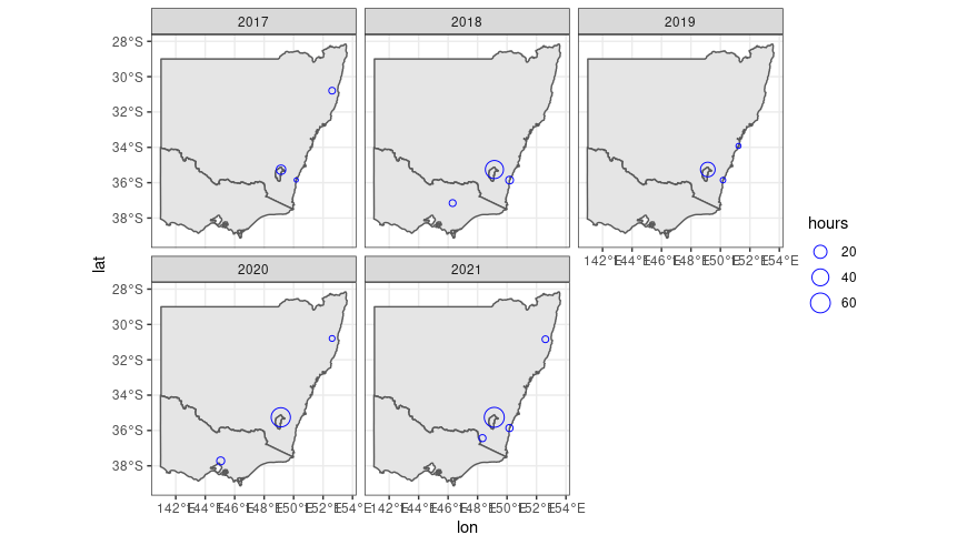
I’ve recently had some fun downloading and displaying my running data from Strava. I’ve been tracking my runs on Strava for the last five years and I thought it would be interesting to make a map showing where I run. Here is one of the plots I made. Each circle is a place in south east Australia where I ran in the given year. The size of the circle corresponds to how many hours I ran there.
I think the plot is a nice visual diary. Looking at the plot, you can see that most of my running took place in my hometown Canberra and that the time I spend running has been increasing. The plot also shows that most years I’ve spent some time running on the south coast and on my grandfather’s farm near Kempsey. You can also see my trips in 2019 and 2020 to the AMSI Summer School. In 2019, the summer school was hosted by UNSW in Sydney and in 2020 it was hosted by La Trobe University in Melbourne. You can also see a circle from this year at Mt Kosciuszko where I ran the Australian Alpine Ascent with my good friend Sarah.
I also made a plot of all my runs on a world map which shows my recent move to California. In this plot all the circles are the same size and I grouped all the runs across the five different years.
I learnt a few things creating these plots and so I thought I would document how I made them.
Creating the plots
Strava lets you download all your data by doing a bulk export. The export includes a zipped folder with all your activities in their original file format.
My activities where saved as .gpx files and I used this handy python library to convert them to .csv files which I could read into R. For the R code I used the packages “tidyverse”, “maps” and “ozmaps”.
Now I had a .csv files for each run. In these files each row corresponded to my location at a given second during the run. What I wanted was a single data frame where each row corresponded to a different run. I found the following way to read in and edit each .csv file:
The first line creates a list of all the .csv files in the working directory. The second line then goes through the list of file names and converts each .csv file into a tibble. I then selected the rows with the time and my location and added a new column with the duration of the run in hours. Finally I removed all the rows except the first row which contains the information about where my run started.
Next I combined these separate tibbles into a single tibble using rbind(). I then added some new columns for grouping the runs. I added a column with the year and columns with the longitude and latitude rounded to the nearest whole number.
To create the plot where you can see where I ran each year, I grouped the runs by the approximate location and by year. I then calculated the total time spent running at each location each year and calculated the average longitude and latitude. I also removed the runs in the USA by only keeping the runs with a negative latitude.
This post is inspired by an assignment question I had to answer for STATS 310A – a probability course at Stanford for first year students in the statistics PhD program. In the question we had to derive a few results about couplings. I found myself thinking and talking about the question long after submitting the assignment and decided to put my thoughts on paper. I would like to thank our lecturer Prof. Diaconis for answering my questions and pointing me in the right direction.
What are couplings?
Given two distribution functions and on , a coupling of and is a distribution function on such that the marginals of are and . Couplings can be used to give probabilistic proofs of analytic statements about and (see here). Couplings are also are studied in their own right in the theory optimal transport.
We can think of and as being the cumulative distribution functions of some random variables and . A coupling of and thus corresponds to a random vector where has the same distribution as , has the same distribution as and .
The independent coupling
For two given distributions function and there exist many possible couplings. For example we could take where . This coupling corresponds to a random vector where and are independent and (as is required for all couplings) , .
In some sense the coupling is in the “middle” of all couplings. This is because and are independent and so doesn’t carry any information about . As the title of the post suggests, there are couplings were this isn’t the case and carries “as much information as possible” about .
The two extremal couplings
Define two function by
and .
With some work, one can show that and are distributions functions on and that they have the correct marginals. In this post I would like to talk about how to construct random vectors and .
Let and be the quantile functions of and . That is,
and .
Now let be a random variable that is uniformly distributed on and define
and .
Since if and only if , we have and likewise . Furthermore occurs if and only if which is equivalent to . Thus
Thus is distributed according to . We see that under the coupling , and are closely related as they are both increasing functions of a common random variable .
We can follow a similar construction for . Define
and .
Thus and are again functions of a common random variable but is an increasing function of and is a decreasing function of . Note that is also uniformly distributed on . Thus and .
Now occurs if and only if and which occurs if and only if . If , then and . On the other hand, if , then and . Thus
,
and so is distributed according to .
What makes and extreme?
Now that we know that and are indeed couplings, it is natural to ask what makes them “extreme”. What we would like to say is that is an increasing function of and is a decreasing function of . Unfortunately this isn’t always the case as can be seen by taking to be constant and to be continuous.
However the intuition that is increasing in and is decreasing in is close to correct. Given a coupling , we can look at the quantity
This quantity tells us something about how changes with . For instance if and were positively correlated, then would be positive and if and were negatively correlated, then would be negative.
For the independent coupling , the quantity is constantly . It turns out that the above probability is maximised by the coupling and minimised by and it is in this sense that they are extremal. This final claim is the two dimensional version of the Fréchet-Hoeffding Theorem and checking it is a good exercise.
The Neyman-Pearson lemma is foundational and important result in the theory of hypothesis testing. When presented in class the proof seemed magical and I had no idea where the ideas came from. I even drew a face like this 😲 next to the usual in my book when the proof was finished. Later in class we learnt the method of undetermined multipliers and suddenly I saw where the Neyman-Pearson lemma came from.
In this blog post, I’ll first give some background and set up notation for the Neyman-Pearson lemma. Then I’ll talk about the method of undetermined multipliers and show how it can be used to derive and prove the Neyman-Pearson lemma. Finally, I’ll write about why I still think the Neyman-Pearson lemma is magical despite the demystified proof.
Background
In the set up of the Neyman-Pearson lemma we have data which is a realisation of some random variable . We wish to conclude something about the distribution of from our data by doing a hypothesis test.
In the Neyman-Pearson lemma we have simple hypotheses. That is our data either comes from the distribution or from the distribution . Thus, our null hypothesis is and our alternative hypothesis is .
A test of against is a function that takes in data and returns a number . The value is the probability under the test of rejecting given the observed data . That is, if , we always reject and if we never reject . For in-between values , we reject with probability .
An ideal test would have two desirable properties. We would like a test that rejects with a low probability when is true but we would also like the test to reject with a high probability when is true. To state this more formally, let and be the expectation of under and respectively. The quantity is the probability we reject when is true. Likewise, the quantity is the probability we reject when is true. An optimal test would be one that minimises and maximises .
Unfortunately the goals of minimising and maximising are at odds with one another. This is because we want to be small in order to minimise and we want to be large to maximise . In nearly all cases we have to trade off between these two goals and there is no single test that simultaneously achieves both.
To work around this, a standard approach is to focus on maximising while requiring that remains below some threshold. The quantity is called the power of the test . If is a number between and , we will say that haslevel– if . A test is said to be most powerful at level-, if
The test is level-.
For all level- tests , the test is more powerful than . That is,
.
Thus we can see that finding a most powerful level- test is a constrained optimisation problem. We wish to maximise the quantity
subject to the constraint
With this in mind, we turn to the method of undetermined multipliers.
The method of undetermined multipliers
The method of undetermined multipliers (also called the method of Lagrange multipliers) is a very general optimisation tool. Suppose that we have a set and two function and we wish to maximise subject to the constraint .
In the context of hypothesis testing, the set is the set of all tests . The objective function is given by . That is, is the power of the test . The constraint function is given by so that if and only if has level-.
The method of undetermined multipliers allows us to reduce this constrained optimisation problem to a (hopefully easier) unconstrained optimisation problem. More specifically we have the following result:
Proposition: Suppose that is such that:
,
There exists , such that maximises over all .
Then maximises under the constraint .
Proof: Suppose that satisfies the above two dot points. We need to show that for all , if , then . By assumption we know that and maximises . Thus, for all ,
.
Now suppose . Then, and so and so as needed.
The constant is the undetermined multiplier. The way to use the method of undetermined is to find values that maximise for each . The multiplier is then varied so that the constraint is satisfied.
Proving the Neyman-Pearson lemma
Now let’s use the method of undetermined multipliers to find most powerful tests. Recall the set which we are optimising over is the set of all tests . Recall also that we wish to optimise subject to the constraint . The method of undetermined multipliers says that we should consider maximising the function
,
where . Suppose that both and have densities1 and with respect to some measure . We can we can write the above expectations as integrals. That is,
and .
Thus the function is equal to
.
We now wish to maximise the function . Recall that is a function that take values in . Thus, the integral
,
is maximised if and only if when and when . Note that if and only if . Thus for each , a test maximises if and only if
The method of undetermined multipliers says that if we can find so that the above is satisfied and , then is a most powerful test. Recall that is equivalent to . By summarising the above argument, we arrive at the Neyman-Pearson lemma,
Neyman-Pearson Lemma2: Suppose that is a test such that
, and
For some ,
then is most powerful at level- for testing against .
The magic of Neyman-Pearson
By learning about undetermined multipliers I’ve been able to better understand the proof of the Neyman-Pearson lemma. I now view it is as clever solution to a constrained optimisation problem rather than something that comes out of nowhere.
There is, however, a different aspect of Neyman-Pearson that continues to surprise me. This aspect is the usefulness of the lemma. At first glance the Neyman-Pearson lemma seems to be a very specialised result because it is about simple hypothesis testing. In reality most interesting hypothesis tests have composite nulls or composite alternatives or both. It turns out that Neyman-Pearson is still incredibly useful for composite testing. Through ideas like monotone likelihood ratios, least favourable distributions and unbiasedness, the Neyman-Pearson lemma or similar ideas can be used to find optimal tests in a variety of settings.
Thus I must admit that the title of this blog post is a little inaccurate and deceptive. I do believe that, given the tools of undetermined multipliers and the set up of simple hypothesis testing, one is naturally led to the Neyman-Pearson lemma. However, I don’t believe that many could have realised how useful and interesting simple hypothesis testing would be.
Footnotes
The assumption that and have densities with respect to a common measure is not a restrictive assumption since one can always take and the apply Radon-Nikodym. However there is often a more natural choice of such as Lebesgue measure on or the counting measure on .
What I call the Neyman-Pearson lemma is really only a third of the Neyman-Pearson lemma. There are two other parts. One that guarantees the existence of a most powerful test and one that is a partial converse to the statement in this post.
Over the course of the past year I have had the pleasure to work with the artist Sanne Carroll on her honours project at the Australian National University. I was one of two mathematics students that collaborated with Sanne. Over the course of the project Sanne drew patterns and would ask Ciaran and I to recreate them using some mathematical or algorithmic ideas. You can see the final version of project here: https://www.sannecarroll.com/ (best viewed on a computer).
I always loved the patterns Sanne drew and the final project is so well put together. Sanne does a great job of incorporating her drawings, the mathematical descriptions and the communication between her, Ciaran and me. Her website building skills also far surpass anything I’ve done on this blog!
It was also a lot of fun to work with Sanne. Hearing about her patterns and talking about maths with her was always fun. I also learnt a few things about GeoGebra which made the animations in my previous post a lot quicker to make. Sanne has told me that she’ll be starting a PhD soon and I’m looking forward to any future collaborations that might arise.


 receives ball 4 followed by ball 5.


 and
and  , and thus
 . Note that if we coloured the balls according to the permutation
  , then we could see that
  .
. 


 .
.


 -double coset. Note however that
  and
and  .
.

 )
)


 given by multiplication by a random transvection (a map of the form
  , where
  ).
). . As Professor Diaconis said, you can’t stop him from taking
  and asking what the resulting random walk on
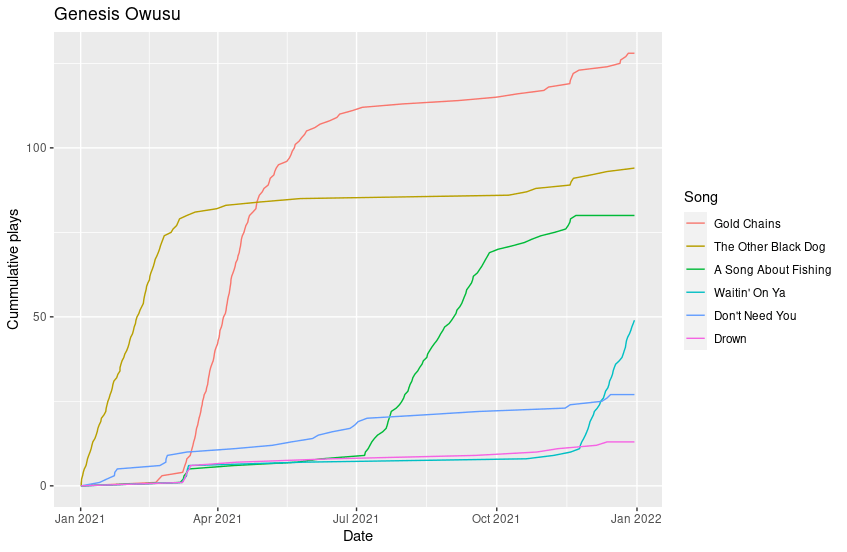
 is a one-dimensional exponential family written in canonical form. That is,
  and there exists a reference measure
  such each distribution
  has a density
  with respect to
 is a sufficient statistic for the model
  . The function
  is the log-partition function for the family
  implies that

 . Thus,
![A'(\theta) = \mathbb{E}_\theta[T(X)]](https://s0.wp.com/latex.php?latex=A%27%28%5Ctheta%29+%3D+%5Cmathbb%7BE%7D_%5Ctheta%5BT%28X%29%5D&bg=ffffff&fg=333333&s=0&c=20201002) , the expectation of
, the expectation of  and we want to use this sample to estimate
  . One way to estimate
 .
.
 solves the equation,
![A'(\widehat{\theta}) = \mathbb{E}_{\widehat{\theta}}[T(X)]](https://s0.wp.com/latex.php?latex=A%27%28%5Cwidehat%7B%5Ctheta%7D%29+%3D+%5Cmathbb%7BE%7D_%7B%5Cwidehat%7B%5Ctheta%7D%7D%5BT%28X%29%5D&bg=ffffff&fg=333333&s=0&c=20201002) . Thus the MLE is the solution to the equation,
. Thus the MLE is the solution to the equation,![\mathbb{E}_{\widehat{\theta}}[T(X)] = \frac{1}{n}\sum_{i=1}^n T(X_i)](https://s0.wp.com/latex.php?latex=%5Cmathbb%7BE%7D_%7B%5Cwidehat%7B%5Ctheta%7D%7D%5BT%28X%29%5D+%3D+%5Cfrac%7B1%7D%7Bn%7D%5Csum_%7Bi%3D1%7D%5En+T%28X_i%29&bg=ffffff&fg=333333&s=0&c=20201002) .
. where
where ![[0,\theta]](https://s0.wp.com/latex.php?latex=%5B0%2C%5Ctheta%5D&bg=ffffff&fg=333333&s=0&c=20201002) . A minimal sufficient statistic for this model is
. A minimal sufficient statistic for this model is  – the maximum of
  . Given what we saw before, we might imague that the MLE for this model would be a method of moments estimator for
  is,
is,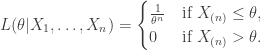
 . However, under
  has a
has a  distribution. Thus,
 ![\mathbb{E}_\theta[X_{(n)}] = \theta \frac{n}{n+1}](https://s0.wp.com/latex.php?latex=%5Cmathbb%7BE%7D_%5Ctheta%5BX_%7B%28n%29%7D%5D++%3D+++%5Ctheta+%5Cfrac%7Bn%7D%7Bn%2B1%7D&bg=ffffff&fg=333333&s=0&c=20201002) so the method of moments estimator would be
so the method of moments estimator would be  .
. .
. be a probability space and let
  be a sub-
 is a random variable
  that satisfies the following two conditions:
 -measurable.
 ,
, ![\mathbb{E}[X1_B] = \mathbb{E}[\mathbb{E}(X|\mathcal{G})1_B]](https://s0.wp.com/latex.php?latex=%5Cmathbb%7BE%7D%5BX1_B%5D+%3D+%5Cmathbb%7BE%7D%5B%5Cmathbb%7BE%7D%28X%7C%5Cmathcal%7BG%7D%291_B%5D&bg=ffffff&fg=333333&s=0&c=20201002) , where
, where  is the indicator function of
  .
. uniformly distributed on the square
 ![[-1,1]^2 \subseteq \mathbb{R}^2](https://s0.wp.com/latex.php?latex=%5B-1%2C1%5D%5E2+%5Csubseteq+%5Cmathbb%7BR%7D%5E2&bg=ffffff&fg=333333&s=0&c=20201002) . Let
. Let  be the unit disc
  . The random variable
  is a simple random variable since
  if
if  and
and  otherwise. Let
  the
the  . It turns out that
  .
. . Since
  is a continuous function of
  for some measurable set
 ![A\subseteq [-1,1]](https://s0.wp.com/latex.php?latex=A%5Csubseteq+%5B-1%2C1%5D&bg=ffffff&fg=333333&s=0&c=20201002) . Thus
. Thus  equals
  and
and ![V \in [-\sqrt{1-U^2}, \sqrt{1-U^2}]](https://s0.wp.com/latex.php?latex=V+%5Cin+%5B-%5Csqrt%7B1-U%5E2%7D%2C+%5Csqrt%7B1-U%5E2%7D%5D&bg=ffffff&fg=333333&s=0&c=20201002) . Since
. Since ![\mathbb{E}[X1_B] = \int_A \int_{-\sqrt{1-u^2}}^{\sqrt{1-u^2}} \frac{1}{4}dvdu = \int_A \frac{1}{2}\sqrt{1-u^2}du](https://s0.wp.com/latex.php?latex=%5Cmathbb%7BE%7D%5BX1_B%5D+%3D+%5Cint_A+%5Cint_%7B-%5Csqrt%7B1-u%5E2%7D%7D%5E%7B%5Csqrt%7B1-u%5E2%7D%7D+%5Cfrac%7B1%7D%7B4%7Ddvdu+%3D+%5Cint_A+%5Cfrac%7B1%7D%7B2%7D%5Csqrt%7B1-u%5E2%7Ddu&bg=ffffff&fg=333333&s=0&c=20201002) .
.![[-1,1]](https://s0.wp.com/latex.php?latex=%5B-1%2C1%5D&bg=ffffff&fg=333333&s=0&c=20201002) and thus has density
and thus has density ![\frac{1}{2}1_{[-1,1]}](https://s0.wp.com/latex.php?latex=%5Cfrac%7B1%7D%7B2%7D1_%7B%5B-1%2C1%5D%7D&bg=ffffff&fg=333333&s=0&c=20201002) . Therefore,
. Therefore,![\mathbb{E}[Y1_B] = \mathbb{E}[\sqrt{1-U^2}1_{\{U \in A\}}] = \int_A \frac{1}{2}\sqrt{1-u^2}du](https://s0.wp.com/latex.php?latex=%5Cmathbb%7BE%7D%5BY1_B%5D+%3D+%5Cmathbb%7BE%7D%5B%5Csqrt%7B1-U%5E2%7D1_%7B%5C%7BU+%5Cin+A%5C%7D%7D%5D+%3D+%5Cint_A+%5Cfrac%7B1%7D%7B2%7D%5Csqrt%7B1-u%5E2%7Ddu&bg=ffffff&fg=333333&s=0&c=20201002) .
.![\mathbb{E}[X1_B] = \mathbb{E}[Y1_B]](https://s0.wp.com/latex.php?latex=%5Cmathbb%7BE%7D%5BX1_B%5D+%3D+%5Cmathbb%7BE%7D%5BY1_B%5D&bg=ffffff&fg=333333&s=0&c=20201002) and therefore
and therefore  , we know that
 ![V \in [-\sqrt{1-u^2},\sqrt{1+u^2}]](https://s0.wp.com/latex.php?latex=V+%5Cin+%5B-%5Csqrt%7B1-u%5E2%7D%2C%5Csqrt%7B1%2Bu%5E2%7D%5D&bg=ffffff&fg=333333&s=0&c=20201002) and that
and that  is uniformly distributed on
 ![[-\sqrt{1-u^2},\sqrt{1+u^2}]](https://s0.wp.com/latex.php?latex=%5B-%5Csqrt%7B1-u%5E2%7D%2C%5Csqrt%7B1%2Bu%5E2%7D%5D&bg=ffffff&fg=333333&s=0&c=20201002) is
is  . Thus given
 ![f:[-1,1]\to \mathbb{R}](https://s0.wp.com/latex.php?latex=f%3A%5B-1%2C1%5D%5Cto+%5Cmathbb%7BR%7D&bg=ffffff&fg=333333&s=0&c=20201002) be any continuous function with
be any continuous function with ![f(x) \in [0,1]](https://s0.wp.com/latex.php?latex=f%28x%29+%5Cin+%5B0%2C1%5D&bg=ffffff&fg=333333&s=0&c=20201002) . With
. With ![A \subseteq [-1,1]^2](https://s0.wp.com/latex.php?latex=A+%5Csubseteq+%5B-1%2C1%5D%5E2&bg=ffffff&fg=333333&s=0&c=20201002) such that
such that  .
. . A climber who came 8th in speed, 1st in bouldering and 2nd in lead climbing would have a lower (and thus better) final score of
  .
.


 and
and  , a coupling of
  such that the marginals of
  where
where  has the same distribution as
  has the same distribution as
  .
. where
where  . This coupling corresponds to a random vector
  where
where  and
and  are independent and (as is required for all couplings)
  ,
,  .
.  is in the “middle” of all couplings. This is because
 ![H_L, H_U :\mathbb{R}^2 \to [0,1]](https://s0.wp.com/latex.php?latex=H_L%2C+H_U+%3A%5Cmathbb%7BR%7D%5E2+%5Cto+%5B0%2C1%5D&bg=ffffff&fg=333333&s=0&c=20201002) by
by and
and  .
. and
and  are distributions functions on
  and
and  .
. and
and  be the quantile functions of
  and
and  .
.![[0,1]](https://s0.wp.com/latex.php?latex=%5B0%2C1%5D&bg=ffffff&fg=333333&s=0&c=20201002) and define
and define and
and  .
. if and only if
  , we have
  and likewise
  . Furthermore
  occurs if and only if
  which is equivalent to
  . Thus
 is distributed according to
  and
and  are closely related as they are both increasing functions of a common random variable
  and
and  .
. and
and  are again functions of a common random variable
  is also uniformly distributed on
  and
and  .
.  occurs if and only if
  which occurs if and only if
  . If
. If  , then
  and
and  . On the other hand, if
  , then
  and
and  . Thus
 ,
, is distributed according to
  , we can look at the quantity
 would be positive and if
  , the quantity
  and it is in this sense that they are extremal. This final claim is the two dimensional version of
  in my book when the proof was finished. Later in class we learnt the method of undetermined multipliers and suddenly I saw where the Neyman-Pearson lemma came from.
  which is a realisation of some random variable
  or from the distribution
  . Thus, our null hypothesis is
  and our alternative hypothesis is
  .
. against
  is a function
  that takes in data
 ![\phi(x) \in [0,1]](https://s0.wp.com/latex.php?latex=%5Cphi%28x%29+%5Cin+%5B0%2C1%5D&bg=ffffff&fg=333333&s=0&c=20201002) . The value
. The value  is the probability under the test
  , we always reject
  we never reject
  , we reject
  .
. ![\mathbb{E}_0[\phi(X)]](https://s0.wp.com/latex.php?latex=%5Cmathbb%7BE%7D_0%5B%5Cphi%28X%29%5D&bg=ffffff&fg=333333&s=0&c=20201002) and
and ![\mathbb{E}_1[\phi(X)]](https://s0.wp.com/latex.php?latex=%5Cmathbb%7BE%7D_1%5B%5Cphi%28X%29%5D&bg=ffffff&fg=333333&s=0&c=20201002) be the expectation of
be the expectation of  under
under  is a number between
 ![\mathbb{E}_1[\phi(X)] \le \alpha](https://s0.wp.com/latex.php?latex=%5Cmathbb%7BE%7D_1%5B%5Cphi%28X%29%5D+%5Cle+%5Calpha&bg=ffffff&fg=333333&s=0&c=20201002) . A test
. A test  , the test
 ![\mathbb{E}_1[\phi'(X)] \le \mathbb{E}_1[\phi(X)]](https://s0.wp.com/latex.php?latex=%5Cmathbb%7BE%7D_1%5B%5Cphi%27%28X%29%5D+%5Cle+%5Cmathbb%7BE%7D_1%5B%5Cphi%28X%29%5D&bg=ffffff&fg=333333&s=0&c=20201002) .
.![\mathbb{E}_0[\phi(X)] \le \alpha](https://s0.wp.com/latex.php?latex=%5Cmathbb%7BE%7D_0%5B%5Cphi%28X%29%5D+%5Cle+%5Calpha&bg=ffffff&fg=333333&s=0&c=20201002)
 and we wish to maximise
  subject to the constraint
  .
.  is given by
 ![f(\phi) = \mathbb{E}_1[\phi(X)]](https://s0.wp.com/latex.php?latex=f%28%5Cphi%29+%3D+%5Cmathbb%7BE%7D_1%5B%5Cphi%28X%29%5D&bg=ffffff&fg=333333&s=0&c=20201002) . That is,
. That is,  is the power of the test
 ![g(\phi)=\mathbb{E}_1[\phi(X)]-\alpha](https://s0.wp.com/latex.php?latex=g%28%5Cphi%29%3D%5Cmathbb%7BE%7D_1%5B%5Cphi%28X%29%5D-%5Calpha&bg=ffffff&fg=333333&s=0&c=20201002) so that
so that  if and only if
  is such that:
  ,
, , such that
  maximises
  over all
  .
. maximises
  . By assumption we know that
  and
and  .
. and so
  and so
  as needed.
  is the undetermined multiplier. The way to use the method of undetermined is to find values
  that maximise
  for each
  is satisfied.
![g(\phi) = \mathbb{E}_0[\phi(X)] - \alpha \le 0](https://s0.wp.com/latex.php?latex=g%28%5Cphi%29+%3D+%5Cmathbb%7BE%7D_0%5B%5Cphi%28X%29%5D+-+%5Calpha+%5Cle+0&bg=ffffff&fg=333333&s=0&c=20201002) . The method of undetermined multipliers says that we should consider maximising the function
. The method of undetermined multipliers says that we should consider maximising the function ![h_k(\phi) = \mathbb{E}_1[\phi(X)] - k\mathbb{E}_0[\phi(X)]](https://s0.wp.com/latex.php?latex=h_k%28%5Cphi%29+%3D+%5Cmathbb%7BE%7D_1%5B%5Cphi%28X%29%5D+-+k%5Cmathbb%7BE%7D_0%5B%5Cphi%28X%29%5D&bg=ffffff&fg=333333&s=0&c=20201002) ,
, and
and ![\mathbb{E}_0[\phi(X)] = \int \phi(x)p_0(x)\mu(dx)](https://s0.wp.com/latex.php?latex=%5Cmathbb%7BE%7D_0%5B%5Cphi%28X%29%5D+%3D+%5Cint+%5Cphi%28x%29p_0%28x%29%5Cmu%28dx%29&bg=ffffff&fg=333333&s=0&c=20201002) and
and ![\mathbb{E}_1[\phi(X)] = \int \phi(x)p_1(x)\mu(dx)](https://s0.wp.com/latex.php?latex=%5Cmathbb%7BE%7D_1%5B%5Cphi%28X%29%5D+%3D+%5Cint+%5Cphi%28x%29p_1%28x%29%5Cmu%28dx%29&bg=ffffff&fg=333333&s=0&c=20201002) .
.  is equal to
 .
. . Recall that
  ,
, when
when  and
and  . Note that
  . Thus for each
  maximises
 , then
  is equivalent to
 ![\mathbb{E}_1[\phi(X)]=\alpha](https://s0.wp.com/latex.php?latex=%5Cmathbb%7BE%7D_1%5B%5Cphi%28X%29%5D%3D%5Calpha&bg=ffffff&fg=333333&s=0&c=20201002) . By summarising the above argument, we arrive at the Neyman-Pearson lemma,
. By summarising the above argument, we arrive at the Neyman-Pearson lemma,![\mathbb{E}_0[\phi(X)] = \alpha](https://s0.wp.com/latex.php?latex=%5Cmathbb%7BE%7D_0%5B%5Cphi%28X%29%5D+%3D+%5Calpha&bg=ffffff&fg=333333&s=0&c=20201002) , and
, and
 and the apply Radon-Nikodym. However there is often a more natural choice of
  or the counting measure on
  .
.