The singular value decomposition (SVD) is a powerful matrix decomposition. It is used all the time in statistics and numerical linear algebra. The SVD is at the heart of the principal component analysis, it demonstrates what’s going on in ridge regression and it is one way to construct the Moore-Penrose inverse of a matrix. For more SVD love, see the tweets below.
In this post I’ll define the SVD and prove that it always exists. At the end we’ll look at some pictures to better understand what’s going on.
Definition
Let  be a
be a  matrix. We will define the singular value decomposition first in the case
  . The SVD consists of three matrix
  and
and  such that
  . The matrix
  is required to be diagonal with non-negative diagonal entries
  . These numbers are called the singular values of . The matrices
  and
and  are required to orthogonal matrices so that
  , the
, the  identity matrix. Note that since is square we also have
  however we won’t have
  unless
  .
.
In the case when  , we can define the SVD of in terms of the SVD of
  . Let
. Let  and
and  be the SVD of so that
  . The SVD of is then given by transposing both sides of this equation giving
  and
and  .
.
Construction
The SVD of a matrix can be found by iteratively solving an optimisation problem. We will first describe an iterative procedure that produces matrices and . We will then verify that  and satisfy the defining properties of the SVD.
We will construct the matrices and one column at a time and we will construct the diagonal matrix one entry at a time. To construct the first columns and entries, recall that the matrix is really a linear function from  to
to  given by
  . We can thus define the operator norm of via

where  represents the Euclidean norm of
  and
and  is the Euclidean norm of
  . The set of vectors
  is a compact set and the function
  is continuous. Thus, the supremum used to define
  is achieved at some vector
  . Define
  . If
. If  , then define
 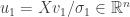 . If
. If  , then define
  to be an arbitrary vector in with
  . To summarise we have
We have now started to fill in our SVD. The number  is the first singular value of and the vectors
  and will be the first columns of the matrices and respectively.
Now suppose that we have found the first  singular values
  and the first columns of and . If
  , then we are done. Otherwise we repeat a similar process.
Let  and
and  be the first columns of and . The vectors split into two subspaces. These subspaces are
  and
and  , the orthogonal compliment of
  . By restricting to
  we get a new linear map
  . Like before, the operator norm of
  is defined to be
 .
.
Since  we must have

The set  is a compact set and thus there exists a vector
  such that
  . As before define
  and
and  if
if  . If
. If  , then define
  to be any vector in
  that is orthogonal to
  .
.
This process repeats until eventually and we have produced matrices and . In the next section, we will argue that these three matrices satisfy the properties of the SVD.
Correctness
The defining properties of the SVD were given at the start of this post. We will see that most of the properties follow immediately from the construction but one of them requires a bit more analysis. Let ![U = [u_1,\ldots,u_p]](https://s0.wp.com/latex.php?latex=U+%3D+%5Bu_1%2C%5Cldots%2Cu_p%5D&bg=ffffff&fg=333333&s=0&c=20201002) ,
,  and
and ![V= [v_1,\ldots,v_p]](https://s0.wp.com/latex.php?latex=V%3D+%5Bv_1%2C%5Cldots%2Cv_p%5D&bg=ffffff&fg=333333&s=0&c=20201002) be the output from the above construction.
be the output from the above construction.
First note that by construction  are orthogonal since we always had
 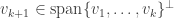 . It follows that the matrix is orthogonal and so
  .
.
The matrix is diagonal by construction. Furthermore, we have that  for every . This is because both
  and
and  were defined as maximum value of over different subsets of . The subset for contained the subset for and thus
  .
.
We’ll next verify that . Since is orthogonal, the vectors  form an orthonormal basis for . It thus suffices to check that
  for
for  . Again by the orthogonality of we have that
  , the
, the  standard basis vector. Thus,

Above, we used that was a diagonal matrix and that  is the column of . If
  , then
  by definition. If
  , then
  and so
  also. Thus, in either case,
  and so
  .
.
The last property we need to verify is that is orthogonal. Note that this isn’t obvious. At each stage of the process, we made sure that . However, in the case that  , we simply defined . It is not clear why this would imply that is orthogonal to .
It turns out that a geometric argument is needed to show this. The idea is that if was not orthogonal to  for some
  , then
  couldn’t have been the value that maximises .
Let  and be two columns of with
  and
and  . We wish to show that
  . To show this we will use the fact that and
  are orthonormal and perform “polar-interpolation“. That is, for
 ![\lambda \in [0,1]](https://s0.wp.com/latex.php?latex=%5Clambda+%5Cin+%5B0%2C1%5D&bg=ffffff&fg=333333&s=0&c=20201002) , define
, define

Since  and are orthogonal, we have that

Furthermore  is orthogonal to
  . Thus, by definition of ,

By the linearity of and the definitions of  ,
,
 .
.
Since  and
and  , we have

Rearranging and dividing by  gives,
 for all
 ![\lambda \in (0,1]](https://s0.wp.com/latex.php?latex=%5Clambda+%5Cin+%280%2C1%5D&bg=ffffff&fg=333333&s=0&c=20201002)
Taking  gives
gives  . Performing the same polar interpolation with
  shows that
  and hence .
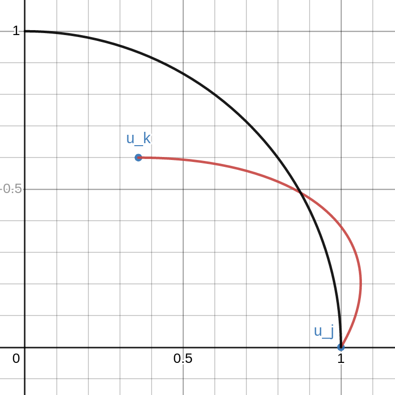
We have thus proved that is orthogonal. This proof is pretty “slick” but it isn’t very illuminating. To better demonstrate the concept, I made an interactive Desmos graph that you can access here.
This graph shows example vectors  . The vector is fixed at
  and a quarter circle of radius
  is drawn. Any vectors
  that are outside this circle have
  .
.
The vector can be moved around inside this quarter circle. This can be done either cby licking and dragging on the point or changing that values of  and
and  on the left. The red curve is the path of
 .
.
As  goes from
  to , the path travels from to .
Note that there is a portion of the red curve near that is outside the black circle. This corresponds to a small value of  that results in
  contradicting the definition of . By moving the point around in the plot you can see that this always happens unless lies exactly on the y-axis. That is, unless is orthogonal to .


instead of
. ↩︎
![U \in [-1,1]](https://s0.wp.com/latex.php?latex=U+%5Cin+%5B-1%2C1%5D&bg=ffffff&fg=333333&s=0&c=20201002) and
and ![V \in [0,1]](https://s0.wp.com/latex.php?latex=V+%5Cin+%5B0%2C1%5D&bg=ffffff&fg=333333&s=0&c=20201002) are independent and uniformly distributed. Then
are independent and uniformly distributed. Then  has the ratio of uniforms distribution. The plot below shows a histogram based on 10,000 samples from the ratio of uniforms distribution
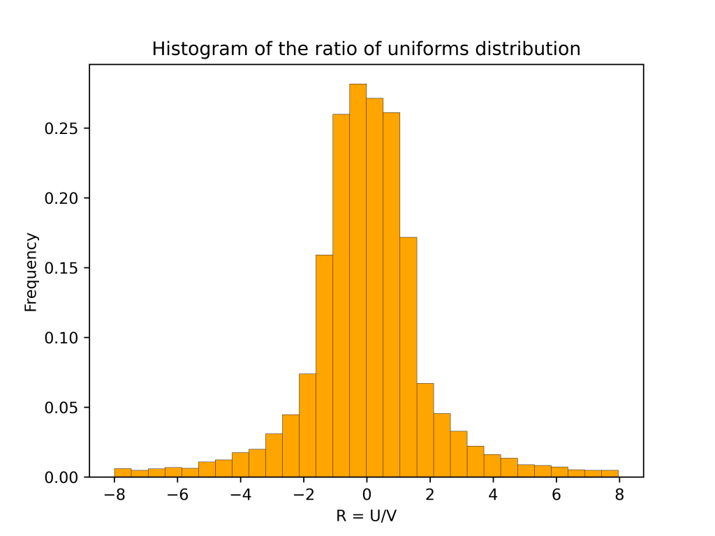
 also has a table mountain shape.


 corresponds to the flat part of the table mountain. The second case corresponds to the sloping curves. The rest of this post use geometry to derive the above formula for
  .
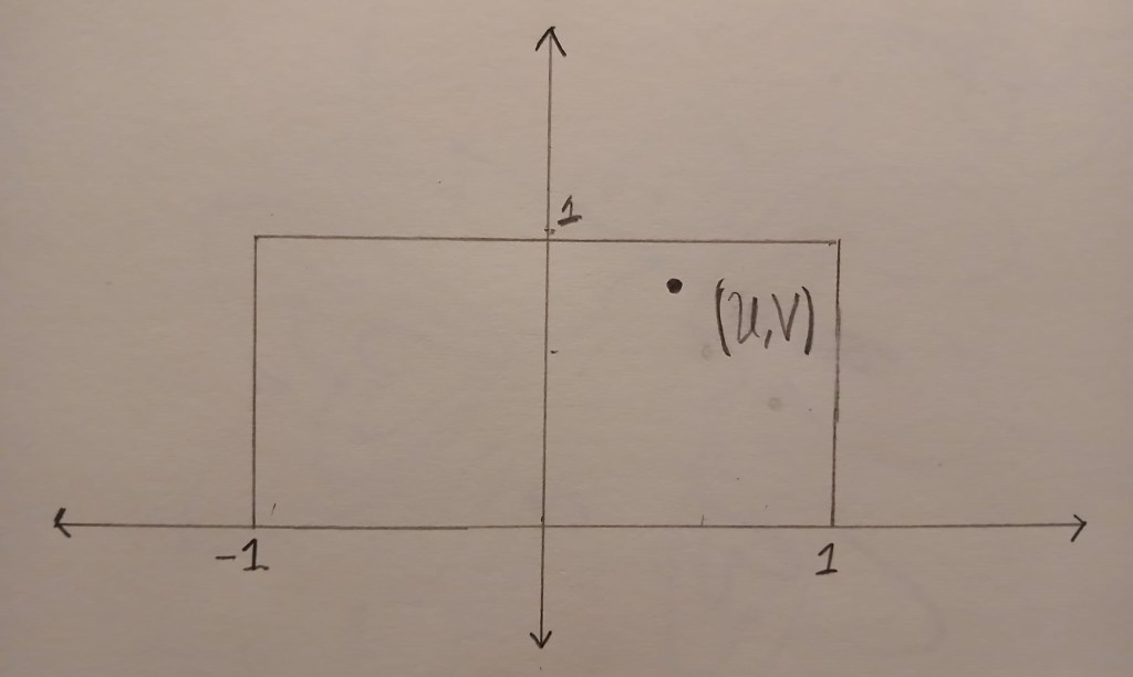
. is uniformly distributed in the box
 ![B=[-1,1] \times [0,1]](https://s0.wp.com/latex.php?latex=B%3D%5B-1%2C1%5D+%5Ctimes+%5B0%2C1%5D&bg=ffffff&fg=333333&s=0&c=20201002) . The image below shows an example of a point
. The image below shows an example of a point  .
.
 and goes through
  . The
. The  .
.
![[R,R+dR]](https://s0.wp.com/latex.php?latex=%5BR%2CR%2BdR%5D&bg=ffffff&fg=333333&s=0&c=20201002) is
is ![\displaystyle{\frac{\text{Area}(\{(u,v) \in B : u/v \in [R, R+dR]\})}{\text{Area}(B)} = \frac{1}{2}\text{Area}(\{(u,v) \in B : u/v \in [R, R+dR]\}).}](https://s0.wp.com/latex.php?latex=%5Cdisplaystyle%7B%5Cfrac%7B%5Ctext%7BArea%7D%28%5C%7B%28u%2Cv%29+%5Cin+B+%3A+u%2Fv+%5Cin+%5BR%2C+R%2BdR%5D%5C%7D%29%7D%7B%5Ctext%7BArea%7D%28B%29%7D+%3D+%5Cfrac%7B1%7D%7B2%7D%5Ctext%7BArea%7D%28%5C%7B%28u%2Cv%29+%5Cin+B+%3A+u%2Fv+%5Cin+%5BR%2C+R%2BdR%5D%5C%7D%29.%7D&bg=ffffff&fg=333333&s=0&c=20201002)
![\displaystyle{h(R) = \lim_{dR \to 0} \frac{1}{2dR}\text{Area}(\{(u,v) \in B : u/v \in [R, R+dR]\})}.](https://s0.wp.com/latex.php?latex=%5Cdisplaystyle%7Bh%28R%29+%3D+%5Clim_%7BdR+%5Cto+0%7D+%5Cfrac%7B1%7D%7B2dR%7D%5Ctext%7BArea%7D%28%5C%7B%28u%2Cv%29+%5Cin+B+%3A+u%2Fv+%5Cin+%5BR%2C+R%2BdR%5D%5C%7D%29%7D.&bg=ffffff&fg=333333&s=0&c=20201002)
 and
and ![\{(u,v) \in B : u/v \in [R, R+dR]\}](https://s0.wp.com/latex.php?latex=%5C%7B%28u%2Cv%29+%5Cin+B+%3A+u%2Fv+%5Cin+%5BR%2C+R%2BdR%5D%5C%7D&bg=ffffff&fg=333333&s=0&c=20201002) is a triangle. This triangle is drawn in blue below.
is a triangle. This triangle is drawn in blue below.
 . The perpendicular height of the triangle from the horizontal edge is
 ![\displaystyle{\text{Area}(\{(u,v) \in B : u/v \in [R, R+dR]\}) =\frac{1}{2}\times dR \times 1=\frac{dR}{2}}.](https://s0.wp.com/latex.php?latex=%5Cdisplaystyle%7B%5Ctext%7BArea%7D%28%5C%7B%28u%2Cv%29+%5Cin+B+%3A+u%2Fv+%5Cin+%5BR%2C+R%2BdR%5D%5C%7D%29+%3D%5Cfrac%7B1%7D%7B2%7D%5Ctimes+dR+%5Ctimes+1%3D%5Cfrac%7BdR%7D%7B2%7D%7D.&bg=ffffff&fg=333333&s=0&c=20201002)
![R \in [-1,1]](https://s0.wp.com/latex.php?latex=R+%5Cin+%5B-1%2C1%5D&bg=ffffff&fg=333333&s=0&c=20201002) we have
we have

 . The perpendicular height of the triangle from the vertical edge is
 ![\displaystyle{\text{Area}(\{(u,v) \in B : u/v \in [R, R+dR]\}) =\frac{1}{2}\times \frac{dR}{R(R+dR)} \times 1=\frac{dR}{2R(R+dR)}}.](https://s0.wp.com/latex.php?latex=%5Cdisplaystyle%7B%5Ctext%7BArea%7D%28%5C%7B%28u%2Cv%29+%5Cin+B+%3A+u%2Fv+%5Cin+%5BR%2C+R%2BdR%5D%5C%7D%29+%3D%5Cfrac%7B1%7D%7B2%7D%5Ctimes+%5Cfrac%7BdR%7D%7BR%28R%2BdR%29%7D+%5Ctimes+1%3D%5Cfrac%7BdR%7D%7B2R%28R%2BdR%29%7D%7D.&bg=ffffff&fg=333333&s=0&c=20201002)

 and
and  . This is because the ratio of uniform distribution has heavy tails. This meant that there were some very large values of
  functions
  and we want to sample from the probability distribution
  That is
 is a normalizing constant. If the set
  is very large, then it may be difficult to compute
  or sample from
  . To approximately sample from
  , we add a auxiliary variable
  such that
 ![\displaystyle{P(U \mid X) = \prod_{i=1}^n \mathrm{Unif}[0,f_i(X)]}.](https://s0.wp.com/latex.php?latex=%5Cdisplaystyle%7BP%28U+%5Cmid+X%29+%3D+%5Cprod_%7Bi%3D1%7D%5En+%5Cmathrm%7BUnif%7D%5B0%2Cf_i%28X%29%5D%7D.&bg=ffffff&fg=333333&s=0&c=20201002)
 are independent and
  is uniformly distributed on the interval
 ![[0,f_i(X)]](https://s0.wp.com/latex.php?latex=%5B0%2Cf_i%28X%29%5D&bg=ffffff&fg=333333&s=0&c=20201002) . If
. If  and
and ![\displaystyle{P(X,U) =P(X)P(U\mid X)\propto \prod_{i=1}^n f_i(X) \frac{1}{f_i(X)} I[U_i \le f(X_i)] = \prod_{i=1}^n I[U_i \le f(X_i)]}.](https://s0.wp.com/latex.php?latex=%5Cdisplaystyle%7BP%28X%2CU%29+%3DP%28X%29P%28U%5Cmid+X%29%5Cpropto++%5Cprod_%7Bi%3D1%7D%5En+f_i%28X%29+%5Cfrac%7B1%7D%7Bf_i%28X%29%7D+I%5BU_i+%5Cle+f%28X_i%29%5D+%3D+%5Cprod_%7Bi%3D1%7D%5En+I%5BU_i+%5Cle+f%28X_i%29%5D%7D.&bg=ffffff&fg=333333&s=0&c=20201002)
 is uniform on the set
 . Then, the above calculation shows that if we discard
  from
from  and then sampling
  from
from  . Since the joint distribution of
  and
and  .
.
 , it might be difficult to do this. Fortunately, there are some notable examples where this step has been worked out. The very first example of auxiliary variables is the Swendsen-Wang algorithm for sampling from the Ising model [2]. In this model it is possible to sample uniformly from
  . Another setting where we can sample exactly is when
  and each
  but an unknown rate
 ![\rho \in [0,1]](https://s0.wp.com/latex.php?latex=%5Crho+%5Cin+%5B0%2C1%5D&bg=ffffff&fg=333333&s=0&c=20201002) . The rate
. The rate  is given a
  prior. That is the prior distribution of
 is a normalizing constant. The model can thus be written as


 .
. . To calculate the distribution of


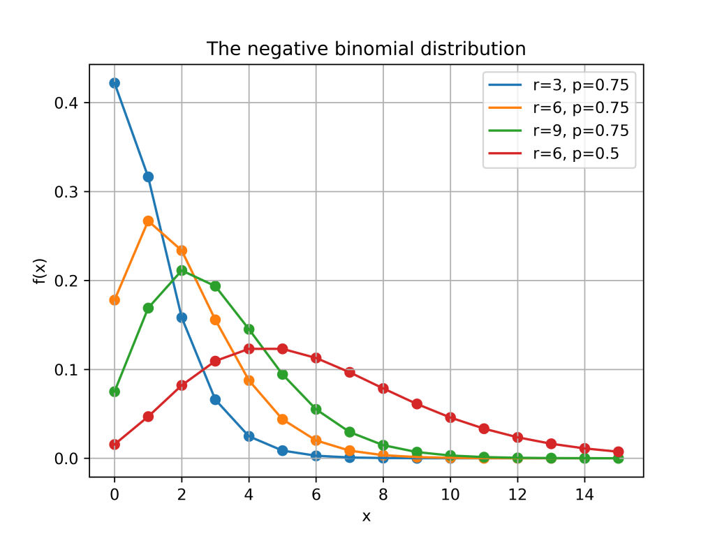
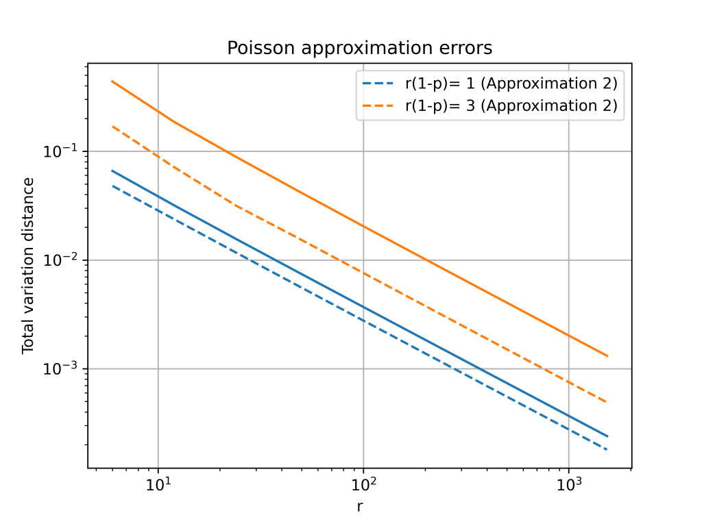
 for
for  and a number of different values of
 and
and  and we want to test if they are from the same distribution. Many popular tests can be reinterpreted as correlation tests by pooling the two samples and introducing a dummy variable that encodes which sample each data point comes from. In this post we will see how this plays out in a simple t-test.
 and
and  , where
  is unknown. Our hypothesis that
  . The test statistic is
 ,
, and
and  are the two sample means. The variable
  is the pooled estimate of the standard deviation and is given by
 .
. follows the T-distribution with
  degrees of freedom. We thus reject the null
  when
when  exceeds the
  quantile of the T-distribution.
  be the pooled data and for
  , define
  by
by 
 can be rewritten as
 . That is, we have expressed our modelling assumptions as a linear model. When working with this linear model, the hypothesis
  . To test
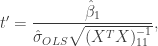
 is the ordinary least squares estimate of
  ,
,  is the design matrix and
  is an estimate of
  given by
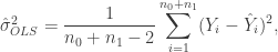
 is the fitted value of
  .
. is exactly equal to
 ![[1,x_i]](https://s0.wp.com/latex.php?latex=%5B1%2Cx_i%5D&bg=ffffff&fg=333333&s=0&c=20201002) and is thus equal to
and is thus equal to


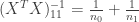 . So,
. So,


 and
and 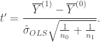
 , we only need to show that
  . To do this, note that the fitted values
  are equal to

 . Therefore,
  and the two sample t-test is equivalent to a correlation test.
 requires creating independent samples
  . The idea is if
  are i.i.d. from
  , then for any test statistic
  , the rank of
  among
among  is uniformly distributed on
  . This means that if
  , then we can reject the hypothesis
  at the significance level
  .
.  is just as intractable as theoretically studying the distribution of
  A Markov chain with transition matrix
 . This means that if
  is a Markov chain with transition matrix
  is distributed according to
  is also distributed according to
  are distributed according to
  from
from 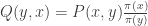 . The transition matrix
  in
in  . That is the chance of drawing
 and let
  be a Markov chain with transition matrix
  be a Markov chain with transition matrix
  ,
, means equal in distribution.
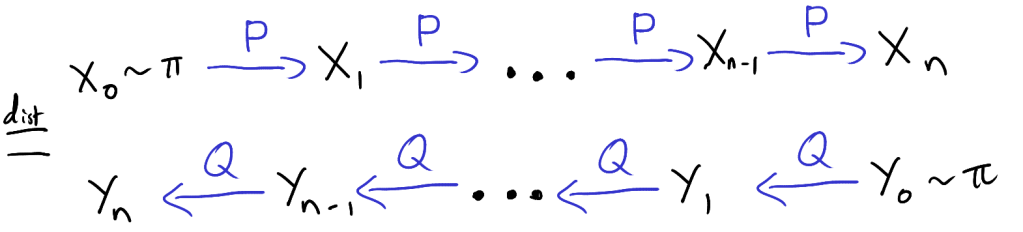
 where
where  is our observed data and
  which we will use to detect outliers. This function is the same function we would use in a regular Monte Carlo test. Namely, we want to reject the null hypothesis when
  is much larger than we would expect under
  uniformly in
  and set
  . We then generate
  as a Markov chain with transition matrix
  as a Markov chain that starts from
 and count the number of
  such that
 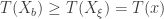 . If there are
  is at most
 .
. 
 does not depend on
  with initial distribution
  independently of
  . This is enough to show that the serial method produces valid p-values. The idea is that since the distribution of
  is in the top
  , let
, let  be the event that
  is in the top
  . That is,
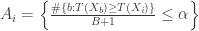 .
. be the indicator function for the event
  values of
  can be in the top
 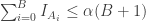 ,
,
 ,
, ,
,  is
is  for all
  .
. .
. . She explains that when an equation says two things are equal we very rarely mean that they are exactly the same thing. What we really mean is that the two things are the same in some ways even though they may be different in others.
  . This is such a familiar statement that you might really think that
  and
and  are the same thing. Indeed, if
  is the same as the number you get when you calculate
  . But calculating
  , then calculating
  but calculating
  is the same as
  .
. and any pair of vectors
  , if
, if  , then
  is invertible and
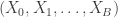
 of size
  that satisfy the above condition.
  and now want the inverse of
  computations since we have to invert a
  matrix. On the right hand side, we only need to compute a small number of matrix-vector products and then add two matrices together. This bring the computational cost down to
  .
.  comes from a distribution of the form:
 ,
, is a vector and
  is equal to the probability that
  are the parameters for the
  ,
, . We can see that the log-likelihood is of the form log-sum-exp. Calculating a log-sum-exp can cause issues with numerical stability. For instance if
  and
and  , for all
  , then the final answer is simply
  . However, as soon as we try to calculate
  on a computer, we’ll be in trouble.
  ,
, .
. we can more safely compute the log-sum-exp expression. For instance, in the
  . This (hopefully) makes each of the terms
  a reasonable size and avoids any numerical issues.
 .
.  . Given a vector
  , the non-central chi-squared distribution with
  is the distribution of the quantity
 . As this notation suggests, the distribution of
  depends only on
  , the norm of
  . The first few times I heard this fact, I had no idea why it would be true (and even found it a little
  such that
  . We wish to show that if
  , then
  .
. have the same norm there exists an orthogonal matrix
  such that
  . Since
  . Furthermore, since
  . This is because, for all
  ,
,
 .
. have the same distribution, we can conclude that
  has the same distribution as
  . Since
  , we are done.
 depends only on the norm of the vector
  and then return
  . But for large values of
  where
where  is the vector with a
 follows the regular chi-squared distribution with
  degrees of freedom and is independent of
  . The regular chi-squared distribution is a special case of the gamma distribution and can be effectively sampled with rejection sampling for large shape parameter (see
  , so for large values of
 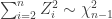 . Finally to get a sample from
  .
. 
 .
. .
. with
with  and
and  .
.