The fundamental theorem of arithmetic states that every natural number can be factorized uniquely as a product of prime numbers. The word “uniquely” here means unique up to rearranging. The theorem means that if you and I take the same number  and I write
  and you write
  where each
  and
and  is a prime number, then in fact
  and we wrote the same prime numbers (but maybe in a different order).
Most people happily accept this theorem as self evident and believe it without proof. Indeed some people take it to be so self evident they feel it doesn’t really deserve the name “theorem” – hence the title of this blog post. In this post I want to highlight two situations where an analogous theorem fails.
Situation One: The Even Numbers
Imagine a world where everything comes in twos. In this world nobody knows of the number one or indeed any odd number. Their counting numbers are the even numbers  . People in this world can add numbers and multiply numbers just like we can. They can even talk about divisibility, for example
  divides
  since
since  . Note that things are already getting a bit strange in this world. Since there is no number one, numbers in this world do not divide themselves.
Once people can talk about divisibility, they can talk about prime numbers. A number is prime in this world if it is not divisible by any other number. For example is prime but as we saw is not prime. Surprisingly the number  is also prime in this world. This is because there are no two even numbers that multiply together to make .
If a number is not prime in this world, we can reduce it to a product of primes. This is because if is not prime, then there are two number  and
and  such that
  . Since
  and are both smaller than , we can apply the same argument and recursively write as a product of primes.
Now we can ask whether or not the fundamental theorem of arthimetic holds in this world. Namely we want to know if their is a unique way to factorize each number in this world. To get an idea we can start with some small even numbers.
- is prime.
 can be factorized uniquely.
- is prime.
 can be factorized uniquely.
 is prime.
 can be factorized uniquely.
 is prime.
 can be factorized uniquely.
 is prime.
 can be factorized uniquely.
Thus it seems as though there might be some hope for this theorem. It at least holds for the first handful of numbers. Unfortunately we eventually get to  and we have:
 and
and  .
.
Thus there are two distinct ways of writing as a product of primes in this world and thus the fundamental theorem of arithmetic does not hold.
Situtation Two: A Number Ring
While the first example is fun and interesting, it is somewhat artificial. We are unlikely to encounter a situation where we only have the even numbers. It is however common and natural for mathematicians to be lead into certain worlds called number rings. We will see one example here and see what an effect the fundamental theorem of arithmetic can have.
Consider wanting to solve the equation  where
where  and
and  are both integers. One way to try to solve this is by rewriting the equation as
  . With this rewriting we have left the familiar world of the whole numbers and entered the number ring
 ![\mathbb{Z}[\sqrt{-19}]](https://s0.wp.com/latex.php?latex=%5Cmathbb%7BZ%7D%5B%5Csqrt%7B-19%7D%5D&bg=ffffff&fg=333333&s=0&c=20201002) .
.
In all numbers have the form  , where and are integers. Addition of two such numbers is defined like so
 .
.
Multiplication is define by using the distributive law and the fact that  . Thus
 .
.
Since we have multiplication we can talk about when a number in divides another and hence define primes in . One can show that if  , then
  and
and  are coprime in (see the references at the end of this post).
This means that there are no primes in that divides both and . If we assume that the fundamental theorem of arthimetic holds in , then this implies that must itself be a cube. This is because  is a cube and if two coprime numbers multiply to be a cube, then both of those coprime numbers must be cubes.
Thus we can conclude that there are integers and such that  . If we expand out this cube we can conclude that
 .
.
Thus in particular we have  . This implies that
  and
and  . Hence
  and
and  . Now if
  , then
  – a contradiction. Similarly if
  , then
  – another contradiction. Thus we can conclude there are no integer solutions to the equation !
Unfortunately however, a bit of searching reveals that  . Thus simply assuming that that the ring has unique factorization led us to incorrectly conclude that an equation had no solutions. The question of unique factorization in number rings such as is a subtle and important one. Some of the flawed proofs of Fermat’s Last Theorem incorrectly assume that certain number rings have unique factorization – like we did above.
References
The lecturer David Smyth showed us that the even integers do not have unique factorization during a lecture of the great course MATH2222.
The example of failing to have unique factorization and the consequences of this was shown in a lecture for a course on algebraic number theory by James Borger. In this class we followed the (freely available) textbook “Number Rings” by P. Stevenhagen. Problem 1.4 on page 8 is the example I used in this post. By viewing the textbook you can see a complete solution to the problem.


instead of
. ↩︎
![U \in [-1,1]](https://s0.wp.com/latex.php?latex=U+%5Cin+%5B-1%2C1%5D&bg=ffffff&fg=333333&s=0&c=20201002) and
and ![V \in [0,1]](https://s0.wp.com/latex.php?latex=V+%5Cin+%5B0%2C1%5D&bg=ffffff&fg=333333&s=0&c=20201002) are independent and uniformly distributed. Then
are independent and uniformly distributed. Then  has the ratio of uniforms distribution. The plot below shows a histogram based on 10,000 samples from the ratio of uniforms distribution
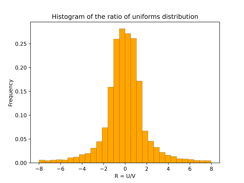
 also has a table mountain shape.


 corresponds to the flat part of the table mountain. The second case corresponds to the sloping curves. The rest of this post use geometry to derive the above formula for
  .
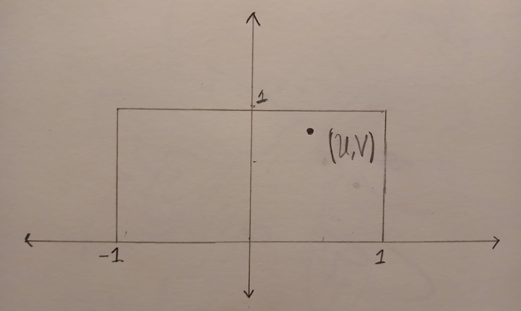
. is uniformly distributed in the box
 ![B=[-1,1] \times [0,1]](https://s0.wp.com/latex.php?latex=B%3D%5B-1%2C1%5D+%5Ctimes+%5B0%2C1%5D&bg=ffffff&fg=333333&s=0&c=20201002) . The image below shows an example of a point
. The image below shows an example of a point  .
.
 and goes through
  . The
. The  .
.
![[R,R+dR]](https://s0.wp.com/latex.php?latex=%5BR%2CR%2BdR%5D&bg=ffffff&fg=333333&s=0&c=20201002) is
is ![\displaystyle{\frac{\text{Area}(\{(u,v) \in B : u/v \in [R, R+dR]\})}{\text{Area}(B)} = \frac{1}{2}\text{Area}(\{(u,v) \in B : u/v \in [R, R+dR]\}).}](https://s0.wp.com/latex.php?latex=%5Cdisplaystyle%7B%5Cfrac%7B%5Ctext%7BArea%7D%28%5C%7B%28u%2Cv%29+%5Cin+B+%3A+u%2Fv+%5Cin+%5BR%2C+R%2BdR%5D%5C%7D%29%7D%7B%5Ctext%7BArea%7D%28B%29%7D+%3D+%5Cfrac%7B1%7D%7B2%7D%5Ctext%7BArea%7D%28%5C%7B%28u%2Cv%29+%5Cin+B+%3A+u%2Fv+%5Cin+%5BR%2C+R%2BdR%5D%5C%7D%29.%7D&bg=ffffff&fg=333333&s=0&c=20201002)
![\displaystyle{h(R) = \lim_{dR \to 0} \frac{1}{2dR}\text{Area}(\{(u,v) \in B : u/v \in [R, R+dR]\})}.](https://s0.wp.com/latex.php?latex=%5Cdisplaystyle%7Bh%28R%29+%3D+%5Clim_%7BdR+%5Cto+0%7D+%5Cfrac%7B1%7D%7B2dR%7D%5Ctext%7BArea%7D%28%5C%7B%28u%2Cv%29+%5Cin+B+%3A+u%2Fv+%5Cin+%5BR%2C+R%2BdR%5D%5C%7D%29%7D.&bg=ffffff&fg=333333&s=0&c=20201002)
 and
and  . In this case, the set
 ![\{(u,v) \in B : u/v \in [R, R+dR]\}](https://s0.wp.com/latex.php?latex=%5C%7B%28u%2Cv%29+%5Cin+B+%3A+u%2Fv+%5Cin+%5BR%2C+R%2BdR%5D%5C%7D&bg=ffffff&fg=333333&s=0&c=20201002) is a triangle. This triangle is drawn in blue below.
is a triangle. This triangle is drawn in blue below.
 . The perpendicular height of the triangle from the horizontal edge is
 ![\displaystyle{\text{Area}(\{(u,v) \in B : u/v \in [R, R+dR]\}) =\frac{1}{2}\times dR \times 1=\frac{dR}{2}}.](https://s0.wp.com/latex.php?latex=%5Cdisplaystyle%7B%5Ctext%7BArea%7D%28%5C%7B%28u%2Cv%29+%5Cin+B+%3A+u%2Fv+%5Cin+%5BR%2C+R%2BdR%5D%5C%7D%29+%3D%5Cfrac%7B1%7D%7B2%7D%5Ctimes+dR+%5Ctimes+1%3D%5Cfrac%7BdR%7D%7B2%7D%7D.&bg=ffffff&fg=333333&s=0&c=20201002)
![R \in [-1,1]](https://s0.wp.com/latex.php?latex=R+%5Cin+%5B-1%2C1%5D&bg=ffffff&fg=333333&s=0&c=20201002) we have
we have

 . The perpendicular height of the triangle from the vertical edge is
 ![\displaystyle{\text{Area}(\{(u,v) \in B : u/v \in [R, R+dR]\}) =\frac{1}{2}\times \frac{dR}{R(R+dR)} \times 1=\frac{dR}{2R(R+dR)}}.](https://s0.wp.com/latex.php?latex=%5Cdisplaystyle%7B%5Ctext%7BArea%7D%28%5C%7B%28u%2Cv%29+%5Cin+B+%3A+u%2Fv+%5Cin+%5BR%2C+R%2BdR%5D%5C%7D%29+%3D%5Cfrac%7B1%7D%7B2%7D%5Ctimes+%5Cfrac%7BdR%7D%7BR%28R%2BdR%29%7D+%5Ctimes+1%3D%5Cfrac%7BdR%7D%7B2R%28R%2BdR%29%7D%7D.&bg=ffffff&fg=333333&s=0&c=20201002)

 and
and  . It is a u-shaped distribution. There are peaks at
  and
and  .
.

 is distributed according to the discrete arcsine distribution with parameter
  converges in distribution to the continuous arcsine distribution on
 ![[0,1]](https://s0.wp.com/latex.php?latex=%5B0%2C1%5D&bg=ffffff&fg=333333&s=0&c=20201002) . The continuous arcsine distribution has the probability density function
. The continuous arcsine distribution has the probability density function
 . It is called the arcsine distribution because the cumulative distribution function involves the arcsine function
 . I was surprised when I was told this, and couldn’t find a reference. The rest of this blog post proves that the discrete arcsine distribution is an instance of the beta-binomial distribution.
 is the Beta-function. To show that the discrete arc sine distribution is an instance of the beta-binomial distribution we need that
  . That is
 ,
, . To prove the above equation, we can first do some simplifying to
  . By definition
 ,
, factorial if
  is a natural number. The Gamma function
  also satisfies the property
  . Using this repeatedly gives

 is the double factorial. The same reasoning gives

 is also equal to the above final expression. Recall
 (and hence
  ). To see why this last claim holds, note that
 as claimed.
 samples to estimate
  , the volume of an

 .
. . That is the distribution
  is an
is an  . The conditional target distribution is
  the uniform distribution on the
  . Here
  is the Kullback-Liebler divergence between
  . Kullback-Liebler divergence is defined as integral. Specifically
 to be the distribution of the norm squared under
  , then
  and likewise for
  . By the rotational symmetry of
 and
and ![r \in [0,1]](https://s0.wp.com/latex.php?latex=r+%5Cin+%5B0%2C1%5D&bg=ffffff&fg=333333&s=0&c=20201002)

 . This means that
  . The distribution
  , then
  is a scaled chi-squared variable. The shape parameter of
  . The density for


 we get that for large
  .
.
 are independent and uniformly distributed on the interval
 ![[-1,1]](https://s0.wp.com/latex.php?latex=%5B-1%2C1%5D&bg=ffffff&fg=333333&s=0&c=20201002) then
then
 with
with  uniform on
  . Next, we count the proportion of vectors
  with
with  . Specifically, if
  is equal to one when

 and the Monte Carlo approximation with
  .
. is even smaller! For example when
  ,
,  . This means that in our one thousand samples we only expect two or three occurrences of the event
  . As a result our estimate has a high variance.
 , the relative error in the approximation is 100%.
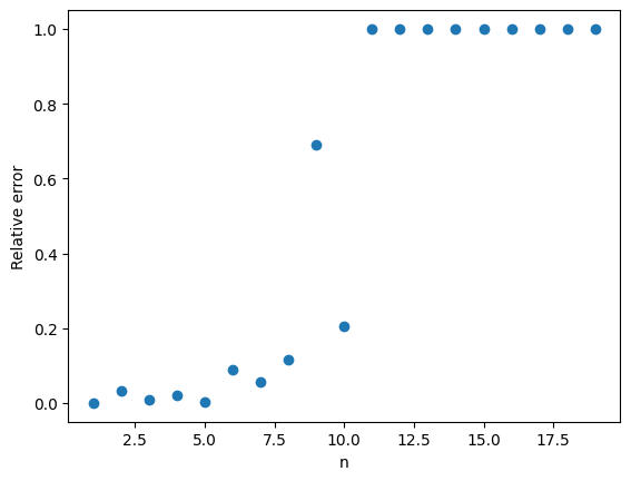
 from the uniform distribution on
  becomes more likely.
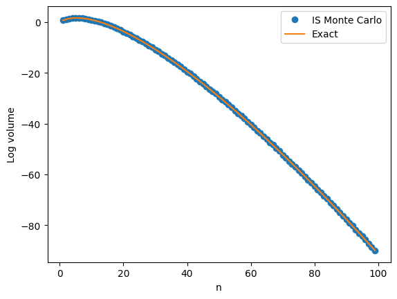
 , we give weights to each of samples and then add up the weights.
  is the density of the proposal distribution, then the IS Monte Carlo estimate of
 and
and  implies
  , the IS Monte Carlo estimate will be an unbiased estimate of
  is one and so the event
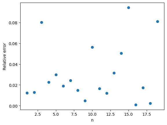
 .
.
 matrix
  is orthogonal if
  . The set of all
  . The uniform distribution on
  is an independent standard normal random variable. Let
  be the columns of
  be the result of applying Gram-Schmidt to
  . Then the matrix
 ![M=[q_1,q_2,\ldots,q_n] \in O_n](https://s0.wp.com/latex.php?latex=M%3D%5Bq_1%2Cq_2%2C%5Cldots%2Cq_n%5D+%5Cin+O_n&bg=ffffff&fg=333333&s=0&c=20201002) is distributed according to Haar measure.
is distributed according to Haar measure. is a QR-factorization of
  is distributed according to Haar measure. However, most numerical libraries do not use Gram-Schmidt to calculate the QR-factorization of a matrix. This means that if you generate a random
 , the top-left entry of a matrix
  . We then compute a diagonal matrix
  with
with  . Then, the matrix
  is Haar distributed. The following python code thus samples a Haar distributed matrix in