This post is an introduction to the negative binomial distribution and a discussion of different ways of approximating the negative binomial distribution.
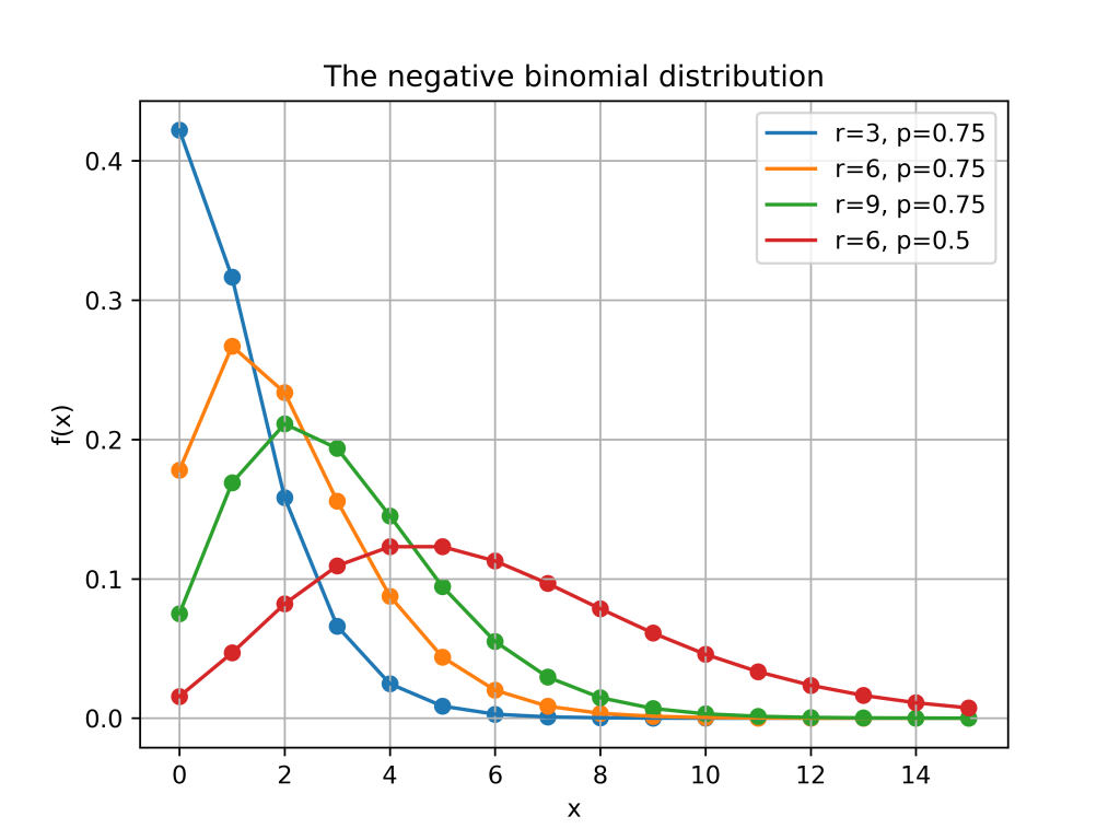
The negative binomial distribution describes the number of times a coin lands on tails before a certain number of heads are recorded. The distribution depends on two parameters and . The parameter is the probability that the coin lands on heads and is the number of heads. If has the negative binomial distribution, then means in the first tosses of the coin, there were heads and that toss number was a head. This means that the probability that is given by
Here is a plot of the function for different values of and .
Poisson approximations
When the parameter is large and is close to one, the negative binomial distribution can be approximated by a Poisson distribution. More formally, suppose that for some positive real number . If is large then, the negative binomial random variable with parameters and , converges to a Poisson random variable with parameter . This is illustrated in the picture below where three negative binomial distributions with approach the Poisson distribution with .
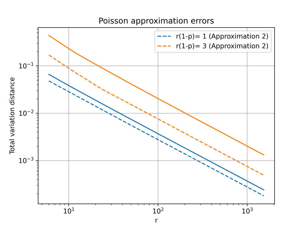
Total variation distance is a common way to measure the distance between two discrete probability distributions. The log-log plot below shows that the error from the Poisson approximation is on the order of and that the error is bigger if the limiting value of is larger.
It turns out that is is possible to get a more accurate approximation by using a different Poisson distribution. In the first approximation, we used a Poisson random variable with mean . However, the mean of the negative binomial distribution is . This suggests that we can get a better approximation by setting .
The change from to is a small because . However, this small change gives a much better approximation, especially for larger values of . The below plot shows that both approximations have errors on the order of , but the constant for the second approximation is much better.
Second order accurate approximation
It is possible to further improve the Poisson approximation by using a Gram–Charlier expansion. A Gram–Charlier approximation for the Poisson distribution is given in this paper.1 The approximation is
where as in the second Poisson approximation and is the Poisson pmf evaluated at .
The Gram–Charlier expansion is considerably more accurate than either Poisson approximation. The errors are on the order of . This higher accuracy means that the error curves for the Gram–Charlier expansion has a steeper slope.
The approximation is given in equation (4) of the paper and is stated in terms of the CDF instead of the PMF. The equation also contains a small typo, it should say instead of . ↩︎
The term “uniformly random” sounds like a contradiction. How can the word “uniform” be used to describe anything that’s random? Uniformly random actually has a precise meaning, and, in a sense, means “as random as possible.” I’ll explain this with an example about shuffling card.
Shuffling cards
Suppose I have a deck of ten cards labeled 1 through 10. Initially, the cards are face down and in perfect order. The card labeled 10 is on top of the deck. The card labeled 9 is second from the top, and so on down to the card labeled 1. The cards are definitely not random.
Next, I generate a random number between 1 and 10. I then find the card with the corresponding label and put it face down on top of the deck. The cards are now somewhat random. The number on top could anything, but the rest of the cards are still in order.The cards are random but they are not uniformly random.
Now suppose that I keep generating random numbers and moving cards to the top of the deck. Each time I do this, the cards get more random. Eventually (after about 30 moves1) the cards will be really jumbled up. Even if you knew the first few cards, it would be hard to predict the order of the remaining ones. Once the cards are really shuffled, they are uniformly random.
Uniformly random
A deck of cards is uniformly random if each of the possible arrangements of the cards are equally likely. After only moving one card, the deck of cards is not uniformly random. This is because there are only 10 possible arrangements of the deck. Once the deck is well-shuffled, all of the 3,628,800 possible arrangements are equally likely.
In general, something is uniformly random if each possibility is equally likely. So the outcome of rolling a fair 6-sided die is uniformly random, but rolling a loaded die is not. The word “uniform” refers to the chance of each possibility (1/6 for each side of the die). These chances are all the same and “uniform”.
This is why uniformly random can mean “as random as possible.” If you are using a fair die or a well-shuffled deck, there are no biases in the outcome. Mathematically, this means you can’t predict the outcome.
Communicating research
The inspiration for this post came from a conversation I had earlier in the week. I was telling someone about my research. As an example, I talked about how long it takes for a deck of cards to become uniformly random. They quickly stopped me and asked how the two words could ever go together. It was a good point! I use the words uniformly random all the time and had never realized this contradiction.2 It was a good reminder about the challenge of clear communication.
Footnotes
The number of moves it takes for the deck to well-shuffled is actually random. But on average it takes around 30 moves. For the mathematical details, see Example 1 in Shuffling Cards and Stopping Times by David Aldous and Persi Diaconis. ↩︎
Of the six posts I published last year, five contain the word uniform! ↩︎
The discrete arcsine distribution is a probability distribution on . It is a u-shaped distribution. There are peaks at and and a dip in the middle. The figure below shows the probability distribution function for .
The probability distribution function of the arcsine distribution is given by
The discrete arcsine distribution is related to simple random walks and to an interesting Markov chain called the Burnside process. The connection with simple random walks is explained in Chapter 3, Volume 1 of An Introduction to Probability and its applications by William Feller. The connection to the Burnside process was discovered by Persi Diaconis in Analysis of a Bose-Einstein Markov Chain.
The discrete arcsine distribution gets its name from the continuous arcsine distribution. Suppose is distributed according to the discrete arcsine distribution with parameter . Then the normalized random variables converges in distribution to the continuous arcsine distribution on . The continuous arcsine distribution has the probability density function
This means that continuous arcsine distribution is a beta distribution with . It is called the arcsine distribution because the cumulative distribution function involves the arcsine function
There is another connection between the discrete and continuous arcsine distributions. The continuous arcsine distribution can be used to sample the discrete arcsine distribution. The two step procedure below produces a sample from the discrete arcsine distribution with parameter :
Sample from the continuous arcsine distribution.
Sample from the binomial distribution with parameters and .
This means that the discrete arcsine distribution is actually the beta-binomial distribution with parameters . I was surprised when I was told this, and couldn’t find a reference. The rest of this blog post proves that the discrete arcsine distribution is an instance of the beta-binomial distribution.
As I showed in this post, the beta-binomial distribution has probability distribution function:
where is the Beta-function. To show that the discrete arc sine distribution is an instance of the beta-binomial distribution we need that . That is
,
for all . To prove the above equation, we can first do some simplifying to . By definition
,
where I have used that factorial if is a natural number. The Gamma function also satisfies the property . Using this repeatedly gives
This means that
where is the double factorial. The same reasoning gives
And so
We’ll now show that is also equal to the above final expression. Recall
And so it suffices to show (and hence ). To see why this last claim holds, note that
Suppose we have two samples and and we want to test if they are from the same distribution. Many popular tests can be reinterpreted as correlation tests by pooling the two samples and introducing a dummy variable that encodes which sample each data point comes from. In this post we will see how this plays out in a simple t-test.
The equal variance t-test
In the equal variance t-test, we assume that and , where is unknown. Our hypothesis that and are from the same distribution becomes the hypothesis . The test statistic is
,
where and are the two sample means. The variable is the pooled estimate of the standard deviation and is given by
.
Under the null hypothesis, follows the T-distribution with degrees of freedom. We thus reject the null when exceeds the quantile of the T-distribution.
Pooling the data
We can turn this two sample test into a correlation test by pooling the data and using a linear model. Let be the pooled data and for , define by
The assumptions that and can be rewritten as
where . That is, we have expressed our modelling assumptions as a linear model. When working with this linear model, the hypothesis is equivalent to . To test we can use the standard t-test for a coefficient in linear model. The test statistic in this case is
where is the ordinary least squares estimate of , is the design matrix and is an estimate of given by
where is the fitted value of .
It turns out that is exactly equal to . We can see this by writing out the design matrix and calculating everything above. The design matrix has rows and is thus equal to
This implies that
And therefore,
Thus, . So,
which is starting to like from the two-sample test. Now
And so
Thus, and
This means to show that , we only need to show that . To do this, note that the fitted values are equal to
Thus,
Which is exactly . Therefore, and the two sample t-test is equivalent to a correlation test.
The Friedman-Rafsky test
In the above example, we saw that the two sample t-test was a special case of the t-test for regressions. This is neat but both tests make very strong assumptions about the data. However, the same thing happens in a more interesting non-parametric setting.
In their 1979 paper, Jerome Friedman and Lawrence Rafsky introduced a two sample tests that makes no assumptions about the distribution of the data. The two samples do not even have to real-valued and can instead be from any metric space. It turns out that their test is a special case of another procedure they devised for testing for association (Friedman & Rafsky, 1983). As with the t-tests above, this connection comes from pooling the two samples and introducing a dummy variable.
The material was based on the discussion and references given in this stackexchange post. The title is a reference to a Halloween lecture on measurability given by Professor Persi Diaconis.
What’s scarier than a non-measurable set?
Making every set measurable. Or rather one particular consequence of making every set measurable.
In my talk, I argued that if you make every set measurable, then there exists a set and an equivalence relation on such that . That is, the set has strictly smaller cardinality than the set of equivalence classes . The contradictory nature of this statement is illustrated in the picture below
We can think of the set as the collection of crosses drawn above. The equivalence relation divides into the regions drawn above. The statement means that in some sense there are more regions than crosses.
To make sense of this we’ll first have to be a bit more precise about what we mean by cardinality.
What do we mean by bigger and smaller?
Let and be two sets. We say that and have the same cardinality and write if there exists a bijection function . We can think of the function as a way of pairing each element of with a unique element of such that every element of is paired with an element of .
We next want to define which means has cardinality at most the cardinality of . There are two reasonable ways in which we could try to define this relationship
We could say means that there exists an injective function .
Alternatively, we could means that there exists a surjective function .
Definitions 1 and 2 say similar things and, in the presence of the axiom of choice, they are equivalent. Since we are going to be making every set measurable in this talk, we won’t be assuming the axiom of choice. Definitions 1 and 2 are thus no longer equivalent and we have a decision to make. We will use definition . in this talk. For justification, note that definition 1 implies that there exists a subset such that . We simply take to be the range of . This is a desirable property of the relation and it’s not clear how this could be done using definition 2.
Infinite binary sequences
It’s time to introduce the set and the equivalence relation we will be working with. The set is the set the set of all function . We can think of each elements as an infinite sequence of zeros and ones stretching off in both directions. For example
.
But this analogy hides something important. Each has a “middle” which is the point . For instance, the two sequences below look the same but when we make bold we see that they are different.
,
.
The equivalence relation on can be thought of as forgetting the location . More formally we have if and only if there exists such that for all . That is, if we shift the sequence by we get the sequence . We will use to denote the equivalence class of and for the set of all equivalences classes.
Some probability
Associated with the space are functions , one for each integer . These functions simply evaluate at . That is . A probabilist or statistician would think of as reporting the result of one of infinitely many independent coin tosses. Normally to make this formal we would have to first define a -algebra on and then define a probability on this -algebra. Today we’re working in a world where every set is measurable and so don’t have to worry about -algebras. Indeed we have the following result:
(Solovay, 1970)1There exists a model of the Zermelo Fraenkel axioms of set theory such that there exists a probability defined on all subsets of such that are i.i.d. .
This result is saying that there is world in which, other than the axiom of choice, all the regular axioms of set theory holds. And in this world, we can assign a probability to every subset in a way so that the events are all independent and have probability . It’s important to note that this is a true countably additive probability and we can apply all our familiar probability results to . We are now ready to state and prove the spooky result claimed at the start of this talk.
Proposition: Given the existence of such a probability , .
Proof: Let be any function. To show that we need to show that is not injective. To do this, we’ll first define another function given by . That is, first maps to ‘s equivalence class and then applies to this equivalence class. This is illustrated below.
A commutative diagram showing the definition of as .
We will show that is almost surely constant with respect to . That is, there exists such that . Each equivalence class is finite or countable and thus has probability zero under . This means that if is almost surely constant, then cannot be injective and must map multiple (in fact infinitely many) equivalence classes to .
It thus remains to show that is almost surely constant. To do this we will introduce a third function . The map is simply the shift map and is given by . Note that and are in the same equivalence class for every . Thus, the map satisfies . That is is -invariant.
The map is ergodic. This means that if satisfies , then equals or . For example if is the event that appears at some point in , then and . Likewise if is the event that the relative frequency of heads converges to a number strictly greater than , then and . The general claim that all -invariant events have probability or can be proved using the independence of .
For each , define an event by . Since is -invariant we have that . Thus, or . This gives us a function given by . Note that for every , . This is because if , then , by definition of . Likewise if , then and hence . Thus, in both cases, .
Since is a probability measure, we can conclude that
.
Thus, map to with probability one. Showing that is almost surely constant and hence that is not injective.
There’s a catch!
So we have proved that there cannot be an injective map . Does this mean we have proved ? Technically no. We have proved the negation of which does not imply . To argue that we need to produce a map that is injective. Surprising this is possible and not too difficult. The idea is to find a map such that implies that . This can be done by somehow encoding in where the centre of is.
A simpler proof and other examples
Our proof was nice because we explicitly calculated the value where sent almost all of . We could have been less explicit and simply noted that the function was measurable with respect to the invariant -algebra of and hence almost surely constant by the ergodicity of .
This quicker proof allows us to generalise our “spooky result” to other sets. Below are two examples where
Fix and define if and only if for some .
if and only if .
A similar argument can be used to show that in Solovay’s world . The exact same argument follows from the ergodicity of the corresponding actions on under the uniform measure.
Three takeaways
I hope you agree that this example is good fun and surprising. I’d like to end with some remarks.
The first remark is some mathematical context. This argument given today is linked to some interesting mathematics called descriptive set theory. This field studies the properties of well behaved subsets (such as Borel subsets) of topological spaces. Descriptive set theory incorporates logic, topology and ergodic theory. I don’t know much about the field but in Persi’s Halloween talk he said that one “monster” was that few people are interested in the subject.
The next remark is a better way to think about our “spooky result”. The result is really saying something about cardinality. When we no longer use the axiom of choice, cardinality becomes a subtle concept. The statement no longer corresponds to being “smaller” than but rather that is “less complex” than . This is perhaps analogous to some statistical models which may be “large” but do not overfit due to subtle constraints on the model complexity.
In light of the previous remark, I would invite you to think about whether the example I gave is truly spookier than non-measurable sets. It might seem to you that it is simply a reasonable consequence of removing the axiom of choice and restricting ourselves to functions we could actually write down or understand. I’ll let you decide
Footnotes
Technically Solovay proved that there exists a model of set theory such that every subset of is Borel measurable. To get the result for binary sequences we have to restrict to and use the binary expansion of to define a function . Solvay’s paper is available here https://www.jstor.org/stable/1970696?seq=1
The fundamental theorem of arithmetic states that every natural number can be factorized uniquely as a product of prime numbers. The word “uniquely” here means unique up to rearranging. The theorem means that if you and I take the same number and I write and you write where each and is a prime number, then in fact and we wrote the same prime numbers (but maybe in a different order).
Most people happily accept this theorem as self evident and believe it without proof. Indeed some people take it to be so self evident they feel it doesn’t really deserve the name “theorem” – hence the title of this blog post. In this post I want to highlight two situations where an analogous theorem fails.
Situation One: The Even Numbers
Imagine a world where everything comes in twos. In this world nobody knows of the number one or indeed any odd number. Their counting numbers are the even numbers . People in this world can add numbers and multiply numbers just like we can. They can even talk about divisibility, for example divides since . Note that things are already getting a bit strange in this world. Since there is no number one, numbers in this world do not divide themselves.
Once people can talk about divisibility, they can talk about prime numbers. A number is prime in this world if it is not divisible by any other number. For example is prime but as we saw is not prime. Surprisingly the number is also prime in this world. This is because there are no two even numbers that multiply together to make .
If a number is not prime in this world, we can reduce it to a product of primes. This is because if is not prime, then there are two number and such that . Since and are both smaller than , we can apply the same argument and recursively write as a product of primes.
Now we can ask whether or not the fundamental theorem of arthimetic holds in this world. Namely we want to know if their is a unique way to factorize each number in this world. To get an idea we can start with some small even numbers.
is prime.
can be factorized uniquely.
is prime.
can be factorized uniquely.
is prime.
can be factorized uniquely.
is prime.
can be factorized uniquely.
is prime.
can be factorized uniquely.
Thus it seems as though there might be some hope for this theorem. It at least holds for the first handful of numbers. Unfortunately we eventually get to and we have:
and .
Thus there are two distinct ways of writing as a product of primes in this world and thus the fundamental theorem of arithmetic does not hold.
Situtation Two: A Number Ring
While the first example is fun and interesting, it is somewhat artificial. We are unlikely to encounter a situation where we only have the even numbers. It is however common and natural for mathematicians to be lead into certain worlds called number rings. We will see one example here and see what an effect the fundamental theorem of arithmetic can have.
Consider wanting to solve the equation where and are both integers. One way to try to solve this is by rewriting the equation as . With this rewriting we have left the familiar world of the whole numbers and entered the number ring .
In all numbers have the form , where and are integers. Addition of two such numbers is defined like so
.
Multiplication is define by using the distributive law and the fact that . Thus
.
Since we have multiplication we can talk about when a number in divides another and hence define primes in . One can show that if , then and are coprime in (see the references at the end of this post).
This means that there are no primes in that divides both and . If we assume that the fundamental theorem of arthimetic holds in , then this implies that must itself be a cube. This is because is a cube and if two coprime numbers multiply to be a cube, then both of those coprime numbers must be cubes.
Thus we can conclude that there are integers and such that . If we expand out this cube we can conclude that
.
Thus in particular we have . This implies that and . Hence and . Now if , then – a contradiction. Similarly if , then – another contradiction. Thus we can conclude there are no integer solutions to the equation !
Unfortunately however, a bit of searching reveals that . Thus simply assuming that that the ring has unique factorization led us to incorrectly conclude that an equation had no solutions. The question of unique factorization in number rings such as is a subtle and important one. Some of the flawed proofs of Fermat’s Last Theorem incorrectly assume that certain number rings have unique factorization – like we did above.
References
The lecturer David Smyth showed us that the even integers do not have unique factorization during a lecture of the great course MATH2222.
The example of failing to have unique factorization and the consequences of this was shown in a lecture for a course on algebraic number theory by James Borger. In this class we followed the (freely available) textbook “Number Rings” by P. Stevenhagen. Problem 1.4 on page 8 is the example I used in this post. By viewing the textbook you can see a complete solution to the problem.


instead of
. ↩︎
 . It is a u-shaped distribution. There are peaks at
  and
and  and a dip in the middle. The figure below shows the probability distribution function for
  .
.

 is distributed according to the discrete arcsine distribution with parameter
  converges in distribution to the continuous arcsine distribution on
 ![[0,1]](https://s0.wp.com/latex.php?latex=%5B0%2C1%5D&bg=ffffff&fg=333333&s=0&c=20201002) . The continuous arcsine distribution has the probability density function
. The continuous arcsine distribution has the probability density function
 . It is called the arcsine distribution because the cumulative distribution function involves the arcsine function
 . I was surprised when I was told this, and couldn’t find a reference. The rest of this blog post proves that the discrete arcsine distribution is an instance of the beta-binomial distribution.
 is the Beta-function. To show that the discrete arc sine distribution is an instance of the beta-binomial distribution we need that
  . That is
 ,
, . To prove the above equation, we can first do some simplifying to
  . By definition
 ,
, factorial if
  is a natural number. The Gamma function
  also satisfies the property
  . Using this repeatedly gives

 is the double factorial. The same reasoning gives

 is also equal to the above final expression. Recall
 (and hence
  ). To see why this last claim holds, note that
 as claimed.
 and
and  and we want to test if they are from the same distribution. Many popular tests can be reinterpreted as correlation tests by pooling the two samples and introducing a dummy variable that encodes which sample each data point comes from. In this post we will see how this plays out in a simple t-test.
 and
and  , where
  is unknown. Our hypothesis that
  . The test statistic is
 ,
, and
and  are the two sample means. The variable
  is the pooled estimate of the standard deviation and is given by
 .
. follows the T-distribution with
  degrees of freedom. We thus reject the null
  when
when  exceeds the
  quantile of the T-distribution.
  be the pooled data and for
  , define
  by
by 
 can be rewritten as
 . That is, we have expressed our modelling assumptions as a linear model. When working with this linear model, the hypothesis
  . To test
 is the ordinary least squares estimate of
  ,
,  is the design matrix and
  is an estimate of
  given by
 is the fitted value of
  .
. is exactly equal to
 ![[1,x_i]](https://s0.wp.com/latex.php?latex=%5B1%2Cx_i%5D&bg=ffffff&fg=333333&s=0&c=20201002) and is thus equal to
and is thus equal to


 . So,
. So,


 and
and 
 , we only need to show that
  . To do this, note that the fitted values
  are equal to

 . Therefore,
  and the two sample t-test is equivalent to a correlation test.
 and an equivalence relation
  on
on  . That is, the set
  . The contradictory nature of this statement is illustrated in the picture below
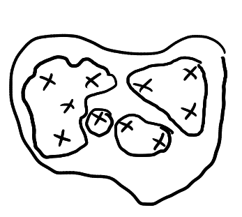
 means that in some sense there are more regions than crosses.
 and
and  be two sets. We say that
  if there exists a bijection function
  . We can think of the function
  as a way of pairing each element of
  which means
  .
. .
. such that
  . We simply take
  to be the range of
  the set of all function
  . We can think of each elements
  as an infinite sequence of zeros and ones stretching off in both directions. For example
 .
. . For instance, the two sequences below look the same but when we make
  ,
, .
. if and only if there exists
  such that
  for all
  . That is, if we shift the sequence
  by
by  . We will use
 ![[\omega]](https://s0.wp.com/latex.php?latex=%5B%5Comega%5D&bg=ffffff&fg=333333&s=0&c=20201002) to denote the equivalence class of
to denote the equivalence class of  , one for each integer
  . That is
  . A probabilist or statistician would think of
  as reporting the result of one of infinitely many independent coin tosses. Normally to make this formal we would have to first define a
  defined on all subsets of
  .
. in a way so that the events
  are all independent and have probability
  . It’s important to note that this is a true countably additive probability and we can apply all our familiar probability results to
  .
. be any function. To show that
  given by
 ![g(\omega)=f([\omega])](https://s0.wp.com/latex.php?latex=g%28%5Comega%29%3Df%28%5B%5Comega%5D%29&bg=ffffff&fg=333333&s=0&c=20201002) . That is,
. That is,  first maps
 is almost surely constant with respect to
  such that
  . Each equivalence class
  .
. is almost surely constant. To do this we will introduce a third function
  . The map
  is simply the shift map and is given by
  . Note that
  are in the same equivalence class for every
  . Thus, the map
  . That is
  , then
  equals
  . For example if
  appears at some point in
  . Likewise if
  . The general claim that all
  by
by  . Since
  . Thus,
  or
or  given by
  . Note that for every
  . This is because if
  , then
  , by definition of
  . Likewise if
  , then
  and hence
  . Thus, in both cases,
  .
. .
.
 . Does this mean we have proved
  ? Technically no. We have proved the negation of
  which does not imply
  . To argue that
  that is injective. Surprising this is possible and not too difficult. The idea is to find a map
  implies that
  . This can be done by somehow encoding in
  where the centre of
 and define
  for some
  .
. is Borel measurable. To get the result for binary sequences we have to restrict to
  and use the binary expansion of
  to define a function
  . Solvay’s paper is available here
  and you write
  where each
  and
and  is a prime number, then in fact
  and we wrote the same prime numbers (but maybe in a different order).
  . People in this world can add numbers and multiply numbers just like we can. They can even talk about divisibility, for example
  divides
  since
since  . Note that things are already getting a bit strange in this world. Since there is no number one, numbers in this world do not divide themselves.
 is also prime in this world. This is because there are no two even numbers that multiply together to make
  and
and  such that
  . Since
  and
and  can be factorized uniquely.
 can be factorized uniquely.
 is prime.
 can be factorized uniquely.
 is prime.
 can be factorized uniquely.
 is prime.
 can be factorized uniquely.
 and we have:
 and
and  .
. where
where  are both integers. One way to try to solve this is by rewriting the equation as
  . With this rewriting we have left the familiar world of the whole numbers and entered the number ring
 ![\mathbb{Z}[\sqrt{-19}]](https://s0.wp.com/latex.php?latex=%5Cmathbb%7BZ%7D%5B%5Csqrt%7B-19%7D%5D&bg=ffffff&fg=333333&s=0&c=20201002) .
.  , where
  .
. . Thus
 .
. , then
  and
and  are coprime in
  is a cube and if two coprime numbers multiply to be a cube, then both of those coprime numbers must be cubes.
 . If we expand out this cube we can conclude that
 .
. . This implies that
  and
and  . Hence
  and
and  . Now if
  , then
  – a contradiction. Similarly if
  , then
  – another contradiction. Thus we can conclude there are no integer solutions to the equation
  . Thus simply assuming that that the ring