This post is an introduction to the negative binomial distribution and a discussion of different ways of approximating the negative binomial distribution.
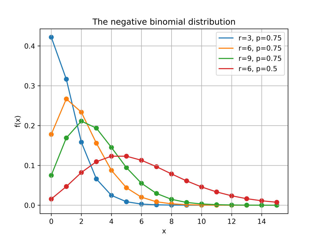
The negative binomial distribution describes the number of times a coin lands on tails before a certain number of heads are recorded. The distribution depends on two parameters and . The parameter is the probability that the coin lands on heads and is the number of heads. If has the negative binomial distribution, then means in the first tosses of the coin, there were heads and that toss number was a head. This means that the probability that is given by
Here is a plot of the function for different values of and .
Poisson approximations
When the parameter is large and is close to one, the negative binomial distribution can be approximated by a Poisson distribution. More formally, suppose that for some positive real number . If is large then, the negative binomial random variable with parameters and , converges to a Poisson random variable with parameter . This is illustrated in the picture below where three negative binomial distributions with approach the Poisson distribution with .
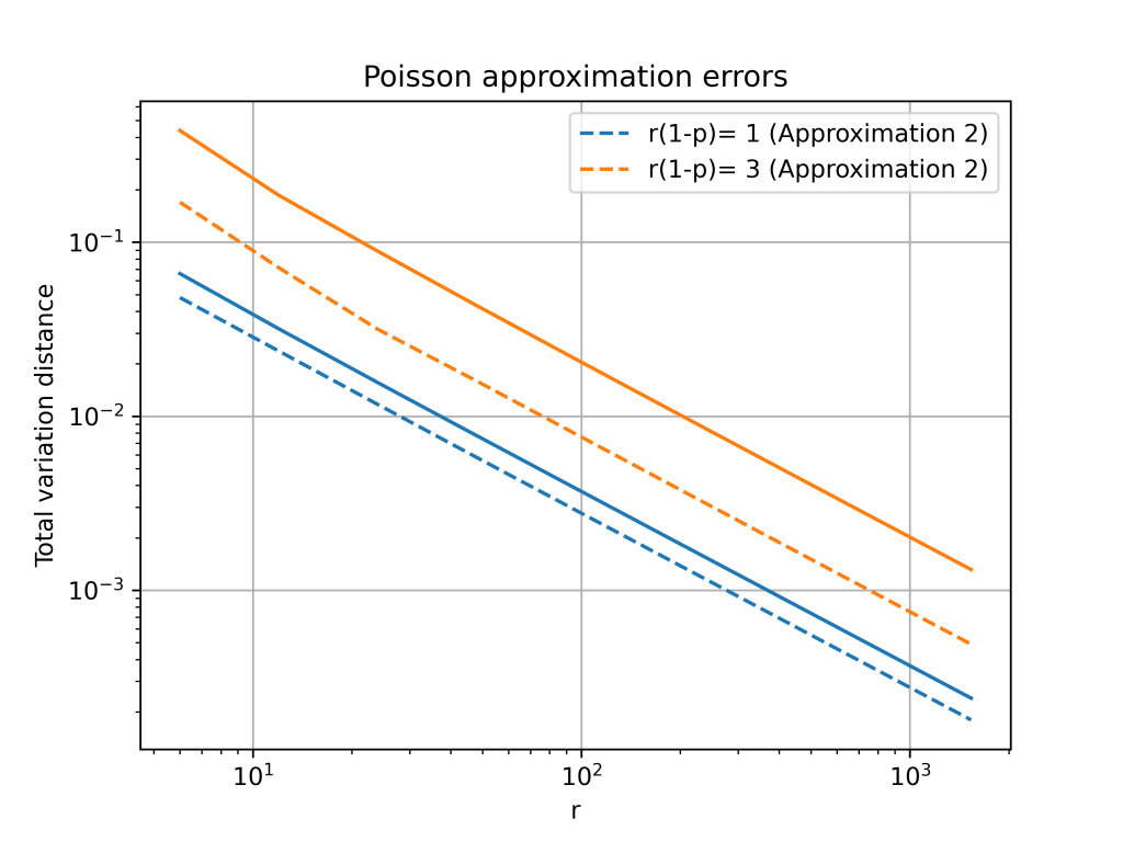
Total variation distance is a common way to measure the distance between two discrete probability distributions. The log-log plot below shows that the error from the Poisson approximation is on the order of and that the error is bigger if the limiting value of is larger.
It turns out that is is possible to get a more accurate approximation by using a different Poisson distribution. In the first approximation, we used a Poisson random variable with mean . However, the mean of the negative binomial distribution is . This suggests that we can get a better approximation by setting .
The change from to is a small because . However, this small change gives a much better approximation, especially for larger values of . The below plot shows that both approximations have errors on the order of , but the constant for the second approximation is much better.
Second order accurate approximation
It is possible to further improve the Poisson approximation by using a Gram–Charlier expansion. A Gram–Charlier approximation for the Poisson distribution is given in this paper.1 The approximation is
where as in the second Poisson approximation and is the Poisson pmf evaluated at .
The Gram–Charlier expansion is considerably more accurate than either Poisson approximation. The errors are on the order of . This higher accuracy means that the error curves for the Gram–Charlier expansion has a steeper slope.
The approximation is given in equation (4) of the paper and is stated in terms of the CDF instead of the PMF. The equation also contains a small typo, it should say instead of . ↩︎
The term “uniformly random” sounds like a contradiction. How can the word “uniform” be used to describe anything that’s random? Uniformly random actually has a precise meaning, and, in a sense, means “as random as possible.” I’ll explain this with an example about shuffling card.
Shuffling cards
Suppose I have a deck of ten cards labeled 1 through 10. Initially, the cards are face down and in perfect order. The card labeled 10 is on top of the deck. The card labeled 9 is second from the top, and so on down to the card labeled 1. The cards are definitely not random.
Next, I generate a random number between 1 and 10. I then find the card with the corresponding label and put it face down on top of the deck. The cards are now somewhat random. The number on top could anything, but the rest of the cards are still in order.The cards are random but they are not uniformly random.
Now suppose that I keep generating random numbers and moving cards to the top of the deck. Each time I do this, the cards get more random. Eventually (after about 30 moves1) the cards will be really jumbled up. Even if you knew the first few cards, it would be hard to predict the order of the remaining ones. Once the cards are really shuffled, they are uniformly random.
Uniformly random
A deck of cards is uniformly random if each of the possible arrangements of the cards are equally likely. After only moving one card, the deck of cards is not uniformly random. This is because there are only 10 possible arrangements of the deck. Once the deck is well-shuffled, all of the 3,628,800 possible arrangements are equally likely.
In general, something is uniformly random if each possibility is equally likely. So the outcome of rolling a fair 6-sided die is uniformly random, but rolling a loaded die is not. The word “uniform” refers to the chance of each possibility (1/6 for each side of the die). These chances are all the same and “uniform”.
This is why uniformly random can mean “as random as possible.” If you are using a fair die or a well-shuffled deck, there are no biases in the outcome. Mathematically, this means you can’t predict the outcome.
Communicating research
The inspiration for this post came from a conversation I had earlier in the week. I was telling someone about my research. As an example, I talked about how long it takes for a deck of cards to become uniformly random. They quickly stopped me and asked how the two words could ever go together. It was a good point! I use the words uniformly random all the time and had never realized this contradiction.2 It was a good reminder about the challenge of clear communication.
Footnotes
The number of moves it takes for the deck to well-shuffled is actually random. But on average it takes around 30 moves. For the mathematical details, see Example 1 in Shuffling Cards and Stopping Times by David Aldous and Persi Diaconis. ↩︎
Of the six posts I published last year, five contain the word uniform! ↩︎
The ratio of uniforms distribution is a useful distribution for rejection sampling. It gives a simple and fast way to sample from discrete distributions like the hypergeometric distribution1. To use the ratio of uniforms distribution in rejection sampling, we need to know the distributions density. This post summarizes some properties of the ratio of uniforms distribution and computes its density.
The ratio of uniforms distribution is the distribution of the ratio of two independent uniform random variables. Specifically, suppose and are independent and uniformly distributed. Then has the ratio of uniforms distribution. The plot below shows a histogram based on 10,000 samples from the ratio of uniforms distribution2.
The histogram has a flat section in the middle and then curves down on either side. This distinctive shape is called a “table mountain”. The density of also has a table mountain shape.
And here is the density plotted on top of the histogram.
A formula for the density of is
The first case in the definition of corresponds to the flat part of the table mountain. The second case corresponds to the sloping curves. The rest of this post use geometry to derive the above formula for .
Calculating the density
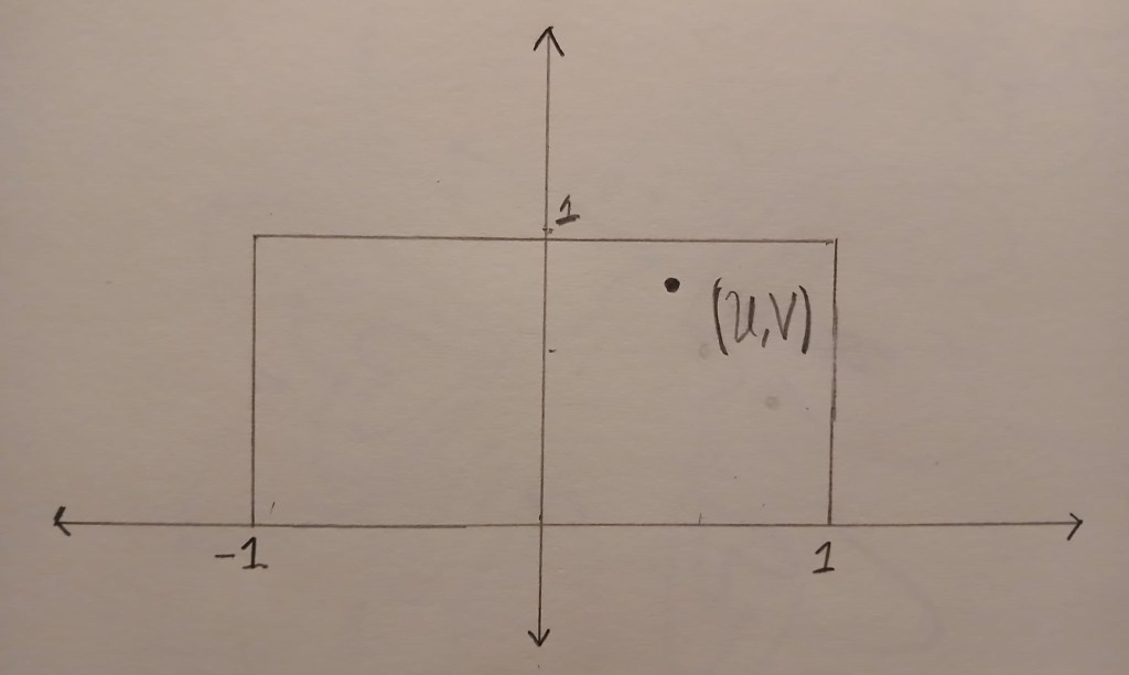
The point is uniformly distributed in the box . The image below shows an example of a point inside the box .
We can compute the ratio geometrically. First we draw a straight line that starts at and goes through . This line will hit the horizontal line . The coordinate at this point is exactly .
In the above picture, all of the points on the dashed line map to the same value of . We can compute the density of by computing an area. The probability that is in a small interval is
If we can compute the above area, then we will know the density of because by definition
We will first work on the case when is between and . In this case, the set is a triangle. This triangle is drawn in blue below.
The horizontal edge of this triangle has length . The perpendicular height of the triangle from the horizontal edge is . This means that
And so, when we have
Now let’s work on the case when is bigger than or less than . In this case, the set is again triangle. But now the triangle has a vertical edge and is much skinnier. Below the triangle is drawn in red. Note that only points inside the box are coloured in.
The vertical edge of the triangle has length . The perpendicular height of the triangle from the vertical edge is . Putting this together
For visual purposes, I restricted the sample to values of between and . This is because the ratio of uniform distribution has heavy tails. This meant that there were some very large values of that made the plot hard to see. ↩︎
The discrete arcsine distribution is a probability distribution on . It is a u-shaped distribution. There are peaks at and and a dip in the middle. The figure below shows the probability distribution function for .
The probability distribution function of the arcsine distribution is given by
The discrete arcsine distribution is related to simple random walks and to an interesting Markov chain called the Burnside process. The connection with simple random walks is explained in Chapter 3, Volume 1 of An Introduction to Probability and its applications by William Feller. The connection to the Burnside process was discovered by Persi Diaconis in Analysis of a Bose-Einstein Markov Chain.
The discrete arcsine distribution gets its name from the continuous arcsine distribution. Suppose is distributed according to the discrete arcsine distribution with parameter . Then the normalized random variables converges in distribution to the continuous arcsine distribution on . The continuous arcsine distribution has the probability density function
This means that continuous arcsine distribution is a beta distribution with . It is called the arcsine distribution because the cumulative distribution function involves the arcsine function
There is another connection between the discrete and continuous arcsine distributions. The continuous arcsine distribution can be used to sample the discrete arcsine distribution. The two step procedure below produces a sample from the discrete arcsine distribution with parameter :
Sample from the continuous arcsine distribution.
Sample from the binomial distribution with parameters and .
This means that the discrete arcsine distribution is actually the beta-binomial distribution with parameters . I was surprised when I was told this, and couldn’t find a reference. The rest of this blog post proves that the discrete arcsine distribution is an instance of the beta-binomial distribution.
As I showed in this post, the beta-binomial distribution has probability distribution function:
where is the Beta-function. To show that the discrete arc sine distribution is an instance of the beta-binomial distribution we need that . That is
,
for all . To prove the above equation, we can first do some simplifying to . By definition
,
where I have used that factorial if is a natural number. The Gamma function also satisfies the property . Using this repeatedly gives
This means that
where is the double factorial. The same reasoning gives
And so
We’ll now show that is also equal to the above final expression. Recall
And so it suffices to show (and hence ). To see why this last claim holds, note that
My last post was about using importance sampling to estimate the volume of high-dimensional ball. The two figures below compare plain Monte Carlo to using importance sampling with a Gaussian proposal. Both plots use samples to estimate , the volume of an -dimensional ball
A friend of mine pointed out that the relative error does not seem to increase with the dimension . He thought it was too good to be true. It turns out he was right and the relative error does increase with dimension but it increases very slowly. To estimate the number of samples needs to grow on the order of .
To prove this, we will use the paper The sample size required for importance sampling by Chatterjee and Diaconis [1]. This paper shows that the sample size for importance sampling is determined by the Kullback-Liebler divergence. The relevant result from their paper is Theorem 1.3. This theorem is about the relative error in using importance sampling to estimate a probability.
In our setting the proposal distribution is . That is the distribution is an -dimensional Gaussian vector with mean and covariance . The conditional target distribution is the uniform distribution on the dimensional ball. Theorem 1.3 in [1] tells us how many samples are needed to estimate . Informally, the required sample size is . Here is the Kullback-Liebler divergence between and .
To use this theorem we need to compute . Kullback-Liebler divergence is defined as integral. Specifically
Computing the high-dimensional integral above looks challenging. Fortunately, it can reduced to a one-dimensional integral. This is because both the distributions and are rotationally symmetric. To use this, define to be the distribution of the norm squared under and . That is if , then and likewise for . By the rotational symmetry of and we have
We can work out both and . The distribution is the uniform distribution on the -dimensional ball. And so for and any
Which implies that has density . This means that is a Beta distribution with parameters . The distribution is a multivariate Gaussian distribution with mean and variance . This means that if , then is a scaled chi-squared variable. The shape parameter of is and scale parameter is . The density for is therefor
The Kullback-Leibler divergence between and is therefor
Getting Mathematica to do the above integral gives
The auxiliary variables sampler is a general Markov chain Monte Carlo (MCMC) technique for sampling from probability distributions with unknown normalizing constants [1, Section 3.1]. Specifically, suppose we have functions and we want to sample from the probability distribution That is
where is a normalizing constant. If the set is very large, then it may be difficult to compute or sample from . To approximately sample from we can run an ergodic Markov chain with as a stationary distribution. Adding auxiliary variables is one way to create such a Markov chain. For each , we add a auxiliary variable such that
That is, conditional on , the auxiliary variables are independent and is uniformly distributed on the interval . If is distributed according to and have the above auxiliary variable distribution, then
This means that the joint distribution of is uniform on the set
Put another way, suppose we could jointly sample from the uniform distribution on . Then, the above calculation shows that if we discard and only keep , then will be sampled from our target distribution .
The auxiliary variables sampler approximately samples from the uniform distribution on is by using a Gibbs sampler. The Gibbs samplers alternates between sampling from and then sampling from . Since the joint distribution of is uniform on , the conditional distributions and are also uniform. The auxiliary variables sampler thus transitions from to according to the two step process
Independently sample uniformly from .
Sample uniformly from the set .
Since the auxiliary variables sampler is based on a Gibbs sampler, we know that the joint distribution of will converge to the uniform distribution on . So when we discard , the distribution of will converge to the target distribution !
Auxiliary variables in practice
To perform step 2 of the auxiliary variables sampler we have to be able to sample uniformly from the sets
Depending on the nature of the set and the functions , it might be difficult to do this. Fortunately, there are some notable examples where this step has been worked out. The very first example of auxiliary variables is the Swendsen-Wang algorithm for sampling from the Ising model [2]. In this model it is possible to sample uniformly from . Another setting where we can sample exactly is when is the real numbers and each is an increasing function of . This is explored in [3] where they apply auxiliary variables to sampling from Bayesian posteriors.
There is an alternative to sampling exactly from the uniform distribution on . Instead of sampling uniformly from , we can run a Markov chain from the old that has the uniform distribution as a stationary distribution. This approach leads to another special case of auxiliary variables which is called “slice sampling” [4].
Suppose you want to calculate an expression of the form
where . Such expressions can be difficult to evaluate directly since the exponentials can easily cause overflow errors. In this post, I’ll talk about a clever way to avoid such errors.
If there were no terms in the second sum we could use the log-sum-exp trick. That is, to calculate
we set and use the identity
Since for all , the left hand side of the above equation can be computed without the risk of overflow. To calculate,
we can use the above method to separately calculate
and
The final result we want is
Since $A > B$, the right hand side of the above expression can be evaluated safely and we will have our final answer.
R code
The R code below defines a function that performs the above procedure
# Safely compute log(sum(exp(pos)) - sum(exp(neg)))
# The default value for neg is an empty vector.

logSumExp <- function(pos, neg = c()){
  max_pos <- max(pos)
  A <- max_pos + log(sum(exp(pos - max_pos)))

  # If neg is empty, the calculation is done
  if (length(neg) == 0){
    return(A)
  }

  # If neg is non-empty, calculate B.
  max_neg <- max(neg)
  B <- max_neg + log(sum(exp(neg - max_neg)))

  # Check that A is bigger than B
  if (A <= B) {
    stop("sum(exp(pos)) must be larger than sum(exp(neg))")
  }

  # log1p() is a built in function that accurately calculates log(1+x) for |x| << 1
  return(A + log1p(-exp(B - A)))
}
An example
The above procedure can be used to evaulate
Evaluating this directly would quickly lead to errors since R (and most other programming languages) cannot compute . However, R has the functions lfactorial() and lchoose() which can compute and for large values of and . We can thus put this expression in the general form at the start of this post
The following R code thus us exactly what we want:
The beta-binomial model is a Bayesian model used to analyze rates. For a great derivation and explanation of this model, I highly recommend watching the second lecture from Richard McElreath’s course Statistical Rethinking. In this model, the data, , is assumed to be binomially distributed with a fixed number of trail but an unknown rate . The rate is given a prior. That is the prior distribution of has a density
where is a normalizing constant. The model can thus be written as
This is a conjugate model, meaning that the posterior distribution of is again a beta distribution. This can be seen by using Bayes rule
The last expression is proportional to a beta density., specifically .
The marginal distribution of
In the above model we are given the distribution of and the conditional distribution of . To calculate the distribution of , we thus need to marginalize over . Specifically,
The term inside the above integral is
Thus,
This distribution is called the beta-binomial distribution. Below is an image from Wikipedia showing a graph of for and a number of different values of and . You can see that, especially for small value of and the distribution is a lot more spread out than the binomial distribution. This is because there is randomness coming from both and the binomial conditional distribution.
Suppose we have two samples and and we want to test if they are from the same distribution. Many popular tests can be reinterpreted as correlation tests by pooling the two samples and introducing a dummy variable that encodes which sample each data point comes from. In this post we will see how this plays out in a simple t-test.
The equal variance t-test
In the equal variance t-test, we assume that and , where is unknown. Our hypothesis that and are from the same distribution becomes the hypothesis . The test statistic is
,
where and are the two sample means. The variable is the pooled estimate of the standard deviation and is given by
.
Under the null hypothesis, follows the T-distribution with degrees of freedom. We thus reject the null when exceeds the quantile of the T-distribution.
Pooling the data
We can turn this two sample test into a correlation test by pooling the data and using a linear model. Let be the pooled data and for , define by
The assumptions that and can be rewritten as
where . That is, we have expressed our modelling assumptions as a linear model. When working with this linear model, the hypothesis is equivalent to . To test we can use the standard t-test for a coefficient in linear model. The test statistic in this case is
where is the ordinary least squares estimate of , is the design matrix and is an estimate of given by
where is the fitted value of .
It turns out that is exactly equal to . We can see this by writing out the design matrix and calculating everything above. The design matrix has rows and is thus equal to
This implies that
And therefore,
Thus, . So,
which is starting to like from the two-sample test. Now
And so
Thus, and
This means to show that , we only need to show that . To do this, note that the fitted values are equal to
Thus,
Which is exactly . Therefore, and the two sample t-test is equivalent to a correlation test.
The Friedman-Rafsky test
In the above example, we saw that the two sample t-test was a special case of the t-test for regressions. This is neat but both tests make very strong assumptions about the data. However, the same thing happens in a more interesting non-parametric setting.
In their 1979 paper, Jerome Friedman and Lawrence Rafsky introduced a two sample tests that makes no assumptions about the distribution of the data. The two samples do not even have to real-valued and can instead be from any metric space. It turns out that their test is a special case of another procedure they devised for testing for association (Friedman & Rafsky, 1983). As with the t-tests above, this connection comes from pooling the two samples and introducing a dummy variable.
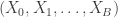
A Monte Carlo significance test of the null hypothesis requires creating independent samples . The idea is if and independently are i.i.d. from , then for any test statistic , the rank of among is uniformly distributed on . This means that if is one of the largest values of , then we can reject the hypothesis at the significance level .
The advantage of Monte Carlo significance tests is that we do not need an analytic expression for the distribution of under . By generating the i.i.d. samples , we are making an empirical distribution that approximates the theoretical distribution. However, sometimes sampling is just as intractable as theoretically studying the distribution of . Often approximate samples based on Markov chain Monte Carlo (MCMC) are used instead. However, these samples are not independent and may not be sampling from the true distribution. This means that a test using MCMC may not be statistically valid
In the 1989 paper Generalized Monte Carlo significance tests, Besag and Clifford propose two methods that solve this exact problem. Their two methods can be used in the same settings where MCMC is used but they are statistically valid and correctly control the Type 1 error. In this post, I will describe just one of the methods – the serial test.
Background on Markov chains
To describe the serial test we will need to introduce some notation. Let denote a transition matrix for a Markov chain on a discrete state space A Markov chain with transition matrix thus satisfies,
Suppose that the transition matrix has a stationary distribution . This means that if is a Markov chain with transition matrix and is distributed according to , then is also distributed according to . This implies that all are distributed according to .
We can construct a new transition matrix from and by . The transition matrix is called the reversal of . This is because for all and in , . That is the chance of drawing from and then transitioning to according to is equal to the chance of drawing from and then transitioning to according to
The new transition matrix also allows us to reverse longer runs of the Markov chain. Fix and let be a Markov chain with transition matrix and initial distribution . Also let be a Markov chain with transition matrix and initial distribution , then
,
where means equal in distribution.
The serial test
Suppose we want to test the hypothesis where is our observed data and is some distribution on . To conduct the serial test, we need to construct a Markov chain for which is a stationary distribution. We then also need to construct the reversal described above. There are many possible ways to construct such as the Metropolis-Hastings algorithm.
We also need a test statistic. This is a function which we will use to detect outliers. This function is the same function we would use in a regular Monte Carlo test. Namely, we want to reject the null hypothesis when is much larger than we would expect under .
The serial test then proceeds as follows. First we pick uniformly in and set . We then generate as a Markov chain with transition matrix that starts at . Likewise we generate as a Markov chain that starts from .
We then apply to each of and count the number of such that . If there are such , then the reported p-value of our test is .
We will now show that this test produces a valid p-value. That is, when , the probability that is less than is at most . In symbols,
Under the null hypothesis , is equal in distribution to generating from and using the transition matrix to go from to .
Thus, under the null hypothesis, the distribution of does not depend on . The entire procedure is equivalent to generating a Markov chain with initial distribution and transition matrix , and then choosing independently of . This is enough to show that the serial method produces valid p-values. The idea is that since the distribution of does not depend on and is uniformly distributed on , the probability that is in the top proportion of should be at most . This is proved more formally below.
For each , let be the event that is in the top proportion of . That is,
.
Let be the indicator function for the event . Since at must values of can be in the top fraction of , we have that
,
Therefor, by linearity of expectations,
By the law of total probability we have,
,
Since is uniform on , is for all . Furthermore, by independence of and , we have
.
Thus, by our previous bound,
.
Applications
In the original paper by Besag and Clifford, the authors discuss how this procedure can be used to perform goodness-of-fit tests. They construct Markov chains that can test the Rasch model or the Ising model. More broadly the method can be used to tests goodness-of-fit tests for any exponential family by using the Markov chains developed by Diaconis and Sturmfels.
A similar method has also been applied more recently to detect Gerrymandering. In this setting, the null hypothesis is the uniform distribution on all valid redistrictings of a state and the test statistics measure the political advantage of a given districting.


instead of
. ↩︎
![U \in [-1,1]](https://s0.wp.com/latex.php?latex=U+%5Cin+%5B-1%2C1%5D&bg=ffffff&fg=333333&s=0&c=20201002) and
and ![V \in [0,1]](https://s0.wp.com/latex.php?latex=V+%5Cin+%5B0%2C1%5D&bg=ffffff&fg=333333&s=0&c=20201002) are independent and uniformly distributed. Then
are independent and uniformly distributed. Then  has the ratio of uniforms distribution. The plot below shows a histogram based on 10,000 samples from the ratio of uniforms distribution
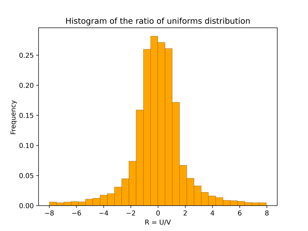
 also has a table mountain shape.


 corresponds to the flat part of the table mountain. The second case corresponds to the sloping curves. The rest of this post use geometry to derive the above formula for
  .
. is uniformly distributed in the box
 ![B=[-1,1] \times [0,1]](https://s0.wp.com/latex.php?latex=B%3D%5B-1%2C1%5D+%5Ctimes+%5B0%2C1%5D&bg=ffffff&fg=333333&s=0&c=20201002) . The image below shows an example of a point
. The image below shows an example of a point  .
.
 and goes through
  . The
. The  .
.
![[R,R+dR]](https://s0.wp.com/latex.php?latex=%5BR%2CR%2BdR%5D&bg=ffffff&fg=333333&s=0&c=20201002) is
is ![\displaystyle{\frac{\text{Area}(\{(u,v) \in B : u/v \in [R, R+dR]\})}{\text{Area}(B)} = \frac{1}{2}\text{Area}(\{(u,v) \in B : u/v \in [R, R+dR]\}).}](https://s0.wp.com/latex.php?latex=%5Cdisplaystyle%7B%5Cfrac%7B%5Ctext%7BArea%7D%28%5C%7B%28u%2Cv%29+%5Cin+B+%3A+u%2Fv+%5Cin+%5BR%2C+R%2BdR%5D%5C%7D%29%7D%7B%5Ctext%7BArea%7D%28B%29%7D+%3D+%5Cfrac%7B1%7D%7B2%7D%5Ctext%7BArea%7D%28%5C%7B%28u%2Cv%29+%5Cin+B+%3A+u%2Fv+%5Cin+%5BR%2C+R%2BdR%5D%5C%7D%29.%7D&bg=ffffff&fg=333333&s=0&c=20201002)
![\displaystyle{h(R) = \lim_{dR \to 0} \frac{1}{2dR}\text{Area}(\{(u,v) \in B : u/v \in [R, R+dR]\})}.](https://s0.wp.com/latex.php?latex=%5Cdisplaystyle%7Bh%28R%29+%3D+%5Clim_%7BdR+%5Cto+0%7D+%5Cfrac%7B1%7D%7B2dR%7D%5Ctext%7BArea%7D%28%5C%7B%28u%2Cv%29+%5Cin+B+%3A+u%2Fv+%5Cin+%5BR%2C+R%2BdR%5D%5C%7D%29%7D.&bg=ffffff&fg=333333&s=0&c=20201002)
 and
and  . In this case, the set
 ![\{(u,v) \in B : u/v \in [R, R+dR]\}](https://s0.wp.com/latex.php?latex=%5C%7B%28u%2Cv%29+%5Cin+B+%3A+u%2Fv+%5Cin+%5BR%2C+R%2BdR%5D%5C%7D&bg=ffffff&fg=333333&s=0&c=20201002) is a triangle. This triangle is drawn in blue below.
is a triangle. This triangle is drawn in blue below.
 . The perpendicular height of the triangle from the horizontal edge is
 ![\displaystyle{\text{Area}(\{(u,v) \in B : u/v \in [R, R+dR]\}) =\frac{1}{2}\times dR \times 1=\frac{dR}{2}}.](https://s0.wp.com/latex.php?latex=%5Cdisplaystyle%7B%5Ctext%7BArea%7D%28%5C%7B%28u%2Cv%29+%5Cin+B+%3A+u%2Fv+%5Cin+%5BR%2C+R%2BdR%5D%5C%7D%29+%3D%5Cfrac%7B1%7D%7B2%7D%5Ctimes+dR+%5Ctimes+1%3D%5Cfrac%7BdR%7D%7B2%7D%7D.&bg=ffffff&fg=333333&s=0&c=20201002)
![R \in [-1,1]](https://s0.wp.com/latex.php?latex=R+%5Cin+%5B-1%2C1%5D&bg=ffffff&fg=333333&s=0&c=20201002) we have
we have

 . The perpendicular height of the triangle from the vertical edge is
 ![\displaystyle{\text{Area}(\{(u,v) \in B : u/v \in [R, R+dR]\}) =\frac{1}{2}\times \frac{dR}{R(R+dR)} \times 1=\frac{dR}{2R(R+dR)}}.](https://s0.wp.com/latex.php?latex=%5Cdisplaystyle%7B%5Ctext%7BArea%7D%28%5C%7B%28u%2Cv%29+%5Cin+B+%3A+u%2Fv+%5Cin+%5BR%2C+R%2BdR%5D%5C%7D%29+%3D%5Cfrac%7B1%7D%7B2%7D%5Ctimes+%5Cfrac%7BdR%7D%7BR%28R%2BdR%29%7D+%5Ctimes+1%3D%5Cfrac%7BdR%7D%7B2R%28R%2BdR%29%7D%7D.&bg=ffffff&fg=333333&s=0&c=20201002)

 and
and  . This is because the ratio of uniform distribution has heavy tails. This meant that there were some very large values of
  . It is a u-shaped distribution. There are peaks at
  and
and  and a dip in the middle. The figure below shows the probability distribution function for
  .
.

 is distributed according to the discrete arcsine distribution with parameter
  converges in distribution to the continuous arcsine distribution on
 ![[0,1]](https://s0.wp.com/latex.php?latex=%5B0%2C1%5D&bg=ffffff&fg=333333&s=0&c=20201002) . The continuous arcsine distribution has the probability density function
. The continuous arcsine distribution has the probability density function
 . It is called the arcsine distribution because the cumulative distribution function involves the arcsine function
 . I was surprised when I was told this, and couldn’t find a reference. The rest of this blog post proves that the discrete arcsine distribution is an instance of the beta-binomial distribution.
 is the Beta-function. To show that the discrete arc sine distribution is an instance of the beta-binomial distribution we need that
  . That is
 ,
, . To prove the above equation, we can first do some simplifying to
  . By definition
 ,
, factorial if
  is a natural number. The Gamma function
  also satisfies the property
  . Using this repeatedly gives

 is the double factorial. The same reasoning gives

 is also equal to the above final expression. Recall
 (and hence
  ). To see why this last claim holds, note that
 as claimed.
 samples to estimate
  , the volume of an

 .
. . That is the distribution
  is an
is an  . The conditional target distribution is
  the uniform distribution on the
  . Here
  is the Kullback-Liebler divergence between
  . Kullback-Liebler divergence is defined as integral. Specifically
 to be the distribution of the norm squared under
  , then
  and likewise for
  . By the rotational symmetry of
 and
and ![r \in [0,1]](https://s0.wp.com/latex.php?latex=r+%5Cin+%5B0%2C1%5D&bg=ffffff&fg=333333&s=0&c=20201002)

 . This means that
  . The distribution
  , then
  is a scaled chi-squared variable. The shape parameter of
  . The density for


 we get that for large
  .
.
 and we want to sample from the probability distribution
  That is
 is a normalizing constant. If the set
  is very large, then it may be difficult to compute
  or sample from
  . To approximately sample from
  , we add a auxiliary variable
  such that
 ![\displaystyle{P(U \mid X) = \prod_{i=1}^n \mathrm{Unif}[0,f_i(X)]}.](https://s0.wp.com/latex.php?latex=%5Cdisplaystyle%7BP%28U+%5Cmid+X%29+%3D+%5Cprod_%7Bi%3D1%7D%5En+%5Cmathrm%7BUnif%7D%5B0%2Cf_i%28X%29%5D%7D.&bg=ffffff&fg=333333&s=0&c=20201002)
 are independent and
  is uniformly distributed on the interval
 ![[0,f_i(X)]](https://s0.wp.com/latex.php?latex=%5B0%2Cf_i%28X%29%5D&bg=ffffff&fg=333333&s=0&c=20201002) . If
. If ![\displaystyle{P(X,U) =P(X)P(U\mid X)\propto \prod_{i=1}^n f_i(X) \frac{1}{f_i(X)} I[U_i \le f(X_i)] = \prod_{i=1}^n I[U_i \le f(X_i)]}.](https://s0.wp.com/latex.php?latex=%5Cdisplaystyle%7BP%28X%2CU%29+%3DP%28X%29P%28U%5Cmid+X%29%5Cpropto++%5Cprod_%7Bi%3D1%7D%5En+f_i%28X%29+%5Cfrac%7B1%7D%7Bf_i%28X%29%7D+I%5BU_i+%5Cle+f%28X_i%29%5D+%3D+%5Cprod_%7Bi%3D1%7D%5En+I%5BU_i+%5Cle+f%28X_i%29%5D%7D.&bg=ffffff&fg=333333&s=0&c=20201002)
 is uniform on the set
 . Then, the above calculation shows that if we discard
  and only keep
  from
from  and then sampling
  from
from  . Since the joint distribution of
  and
and  .
.
 , it might be difficult to do this. Fortunately, there are some notable examples where this step has been worked out. The very first example of auxiliary variables is the Swendsen-Wang algorithm for sampling from the Ising model [2]. In this model it is possible to sample uniformly from
  . Another setting where we can sample exactly is when
  and each
 . Such expressions can be difficult to evaluate directly since the exponentials can easily cause overflow errors. In this post, I’ll talk about a clever way to avoid such errors.
 and use the identity
 for all
  , the left hand side of the above equation can be computed without the risk of overflow. To calculate,
 and
and 

 . However, R has the functions
  and
and  for large values of
  and
and 
 but an unknown rate
 ![\rho \in [0,1]](https://s0.wp.com/latex.php?latex=%5Crho+%5Cin+%5B0%2C1%5D&bg=ffffff&fg=333333&s=0&c=20201002) . The rate
. The rate  is given a
  prior. That is the prior distribution of
 is a normalizing constant. The model can thus be written as


 .
. . To calculate the distribution of


 for
for  and a number of different values of
  and
and  . You can see that, especially for small value of
 and
and  and we want to test if they are from the same distribution. Many popular tests can be reinterpreted as correlation tests by pooling the two samples and introducing a dummy variable that encodes which sample each data point comes from. In this post we will see how this plays out in a simple t-test.
 and
and  , where
  is unknown. Our hypothesis that
  . The test statistic is
 ,
, and
and  are the two sample means. The variable
  is the pooled estimate of the standard deviation and is given by
 .
. follows the T-distribution with
  degrees of freedom. We thus reject the null
  when
when  exceeds the
  quantile of the T-distribution.
  be the pooled data and for
  , define
  by
by 
 can be rewritten as
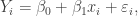
 . That is, we have expressed our modelling assumptions as a linear model. When working with this linear model, the hypothesis
  . To test
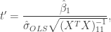
 is the ordinary least squares estimate of
  ,
,  is the design matrix and
  is an estimate of
  given by
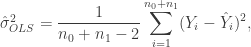
 is the fitted value of
  .
. is exactly equal to
 ![[1,x_i]](https://s0.wp.com/latex.php?latex=%5B1%2Cx_i%5D&bg=ffffff&fg=333333&s=0&c=20201002) and is thus equal to
and is thus equal to


 . So,
. So,


 and
and 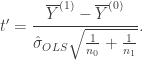
 , we only need to show that
  . To do this, note that the fitted values
  are equal to

 . Therefore,
  and the two sample t-test is equivalent to a correlation test.
 requires creating independent samples
  . The idea is if
  are i.i.d. from
  , then for any test statistic
  , the rank of
  among
among  is uniformly distributed on
  . This means that if
  largest values of
  , then we can reject the hypothesis
  at the significance level
  .
.  is just as intractable as theoretically studying the distribution of
  A Markov chain with transition matrix
 . This means that if
  is a Markov chain with transition matrix
  is distributed according to
  is also distributed according to
  are distributed according to
 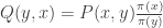 . The transition matrix
  in
in  . That is the chance of drawing
 and let
  be a Markov chain with transition matrix
  be a Markov chain with transition matrix
  ,
, means equal in distribution.
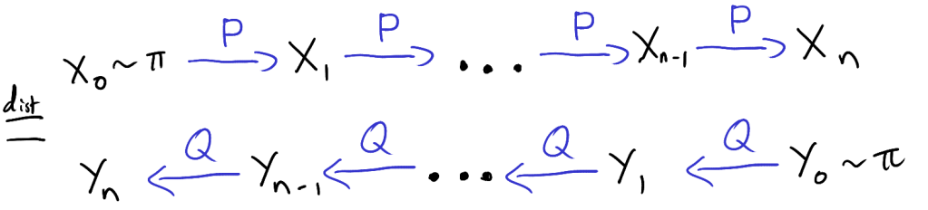
 where
where  is our observed data and
  which we will use to detect outliers. This function is the same function we would use in a regular Monte Carlo test. Namely, we want to reject the null hypothesis when
  is much larger than we would expect under
  uniformly in
  and set
  . We then generate
  as a Markov chain with transition matrix
  as a Markov chain that starts from
 and count the number of
  such that
 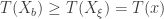 . If there are
  is at most
 .
. 
 does not depend on
  with initial distribution
  independently of
  . This is enough to show that the serial method produces valid p-values. The idea is that since the distribution of
  is in the top
  , let
, let  be the event that
  is in the top
  . That is,
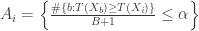 .
. be the indicator function for the event
  values of
 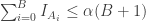 ,
,
 ,
, ,
,  is
is  for all
  .
. .
.