This post is an introduction to the negative binomial distribution and a discussion of different ways of approximating the negative binomial distribution.
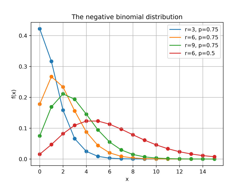
The negative binomial distribution describes the number of times a coin lands on tails before a certain number of heads are recorded. The distribution depends on two parameters and . The parameter is the probability that the coin lands on heads and is the number of heads. If has the negative binomial distribution, then means in the first tosses of the coin, there were heads and that toss number was a head. This means that the probability that is given by
Here is a plot of the function for different values of and .
Poisson approximations
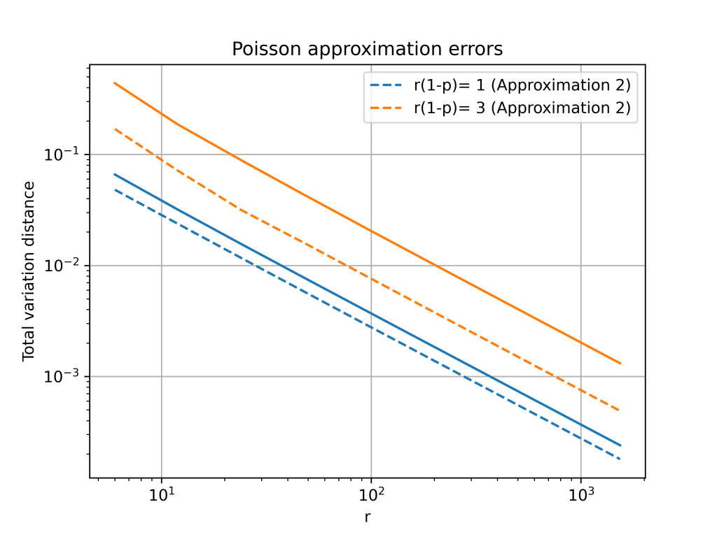
When the parameter is large and is close to one, the negative binomial distribution can be approximated by a Poisson distribution. More formally, suppose that for some positive real number . If is large then, the negative binomial random variable with parameters and , converges to a Poisson random variable with parameter . This is illustrated in the picture below where three negative binomial distributions with approach the Poisson distribution with .
Total variation distance is a common way to measure the distance between two discrete probability distributions. The log-log plot below shows that the error from the Poisson approximation is on the order of and that the error is bigger if the limiting value of is larger.
It turns out that is is possible to get a more accurate approximation by using a different Poisson distribution. In the first approximation, we used a Poisson random variable with mean . However, the mean of the negative binomial distribution is . This suggests that we can get a better approximation by setting .
The change from to is a small because . However, this small change gives a much better approximation, especially for larger values of . The below plot shows that both approximations have errors on the order of , but the constant for the second approximation is much better.
Second order accurate approximation
It is possible to further improve the Poisson approximation by using a Gram–Charlier expansion. A Gram–Charlier approximation for the Poisson distribution is given in this paper.1 The approximation is
where as in the second Poisson approximation and is the Poisson pmf evaluated at .
The Gram–Charlier expansion is considerably more accurate than either Poisson approximation. The errors are on the order of . This higher accuracy means that the error curves for the Gram–Charlier expansion has a steeper slope.
The approximation is given in equation (4) of the paper and is stated in terms of the CDF instead of the PMF. The equation also contains a small typo, it should say instead of . ↩︎
The term “uniformly random” sounds like a contradiction. How can the word “uniform” be used to describe anything that’s random? Uniformly random actually has a precise meaning, and, in a sense, means “as random as possible.” I’ll explain this with an example about shuffling card.
Shuffling cards
Suppose I have a deck of ten cards labeled 1 through 10. Initially, the cards are face down and in perfect order. The card labeled 10 is on top of the deck. The card labeled 9 is second from the top, and so on down to the card labeled 1. The cards are definitely not random.
Next, I generate a random number between 1 and 10. I then find the card with the corresponding label and put it face down on top of the deck. The cards are now somewhat random. The number on top could anything, but the rest of the cards are still in order.The cards are random but they are not uniformly random.
Now suppose that I keep generating random numbers and moving cards to the top of the deck. Each time I do this, the cards get more random. Eventually (after about 30 moves1) the cards will be really jumbled up. Even if you knew the first few cards, it would be hard to predict the order of the remaining ones. Once the cards are really shuffled, they are uniformly random.
Uniformly random
A deck of cards is uniformly random if each of the possible arrangements of the cards are equally likely. After only moving one card, the deck of cards is not uniformly random. This is because there are only 10 possible arrangements of the deck. Once the deck is well-shuffled, all of the 3,628,800 possible arrangements are equally likely.
In general, something is uniformly random if each possibility is equally likely. So the outcome of rolling a fair 6-sided die is uniformly random, but rolling a loaded die is not. The word “uniform” refers to the chance of each possibility (1/6 for each side of the die). These chances are all the same and “uniform”.
This is why uniformly random can mean “as random as possible.” If you are using a fair die or a well-shuffled deck, there are no biases in the outcome. Mathematically, this means you can’t predict the outcome.
Communicating research
The inspiration for this post came from a conversation I had earlier in the week. I was telling someone about my research. As an example, I talked about how long it takes for a deck of cards to become uniformly random. They quickly stopped me and asked how the two words could ever go together. It was a good point! I use the words uniformly random all the time and had never realized this contradiction.2 It was a good reminder about the challenge of clear communication.
Footnotes
The number of moves it takes for the deck to well-shuffled is actually random. But on average it takes around 30 moves. For the mathematical details, see Example 1 in Shuffling Cards and Stopping Times by David Aldous and Persi Diaconis. ↩︎
Of the six posts I published last year, five contain the word uniform! ↩︎
The ratio of uniforms distribution is a useful distribution for rejection sampling. It gives a simple and fast way to sample from discrete distributions like the hypergeometric distribution1. To use the ratio of uniforms distribution in rejection sampling, we need to know the distributions density. This post summarizes some properties of the ratio of uniforms distribution and computes its density.
The ratio of uniforms distribution is the distribution of the ratio of two independent uniform random variables. Specifically, suppose and are independent and uniformly distributed. Then has the ratio of uniforms distribution. The plot below shows a histogram based on 10,000 samples from the ratio of uniforms distribution2.
The histogram has a flat section in the middle and then curves down on either side. This distinctive shape is called a “table mountain”. The density of also has a table mountain shape.
And here is the density plotted on top of the histogram.
A formula for the density of is
The first case in the definition of corresponds to the flat part of the table mountain. The second case corresponds to the sloping curves. The rest of this post use geometry to derive the above formula for .
Calculating the density
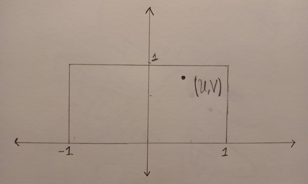
The point is uniformly distributed in the box . The image below shows an example of a point inside the box .
We can compute the ratio geometrically. First we draw a straight line that starts at and goes through . This line will hit the horizontal line . The coordinate at this point is exactly .
In the above picture, all of the points on the dashed line map to the same value of . We can compute the density of by computing an area. The probability that is in a small interval is
If we can compute the above area, then we will know the density of because by definition
We will first work on the case when is between and . In this case, the set is a triangle. This triangle is drawn in blue below.
The horizontal edge of this triangle has length . The perpendicular height of the triangle from the horizontal edge is . This means that
And so, when we have
Now let’s work on the case when is bigger than or less than . In this case, the set is again triangle. But now the triangle has a vertical edge and is much skinnier. Below the triangle is drawn in red. Note that only points inside the box are coloured in.
The vertical edge of the triangle has length . The perpendicular height of the triangle from the vertical edge is . Putting this together
For visual purposes, I restricted the sample to values of between and . This is because the ratio of uniform distribution has heavy tails. This meant that there were some very large values of that made the plot hard to see. ↩︎
The discrete arcsine distribution is a probability distribution on . It is a u-shaped distribution. There are peaks at and and a dip in the middle. The figure below shows the probability distribution function for .
The probability distribution function of the arcsine distribution is given by
The discrete arcsine distribution is related to simple random walks and to an interesting Markov chain called the Burnside process. The connection with simple random walks is explained in Chapter 3, Volume 1 of An Introduction to Probability and its applications by William Feller. The connection to the Burnside process was discovered by Persi Diaconis in Analysis of a Bose-Einstein Markov Chain.
The discrete arcsine distribution gets its name from the continuous arcsine distribution. Suppose is distributed according to the discrete arcsine distribution with parameter . Then the normalized random variables converges in distribution to the continuous arcsine distribution on . The continuous arcsine distribution has the probability density function
This means that continuous arcsine distribution is a beta distribution with . It is called the arcsine distribution because the cumulative distribution function involves the arcsine function
There is another connection between the discrete and continuous arcsine distributions. The continuous arcsine distribution can be used to sample the discrete arcsine distribution. The two step procedure below produces a sample from the discrete arcsine distribution with parameter :
Sample from the continuous arcsine distribution.
Sample from the binomial distribution with parameters and .
This means that the discrete arcsine distribution is actually the beta-binomial distribution with parameters . I was surprised when I was told this, and couldn’t find a reference. The rest of this blog post proves that the discrete arcsine distribution is an instance of the beta-binomial distribution.
As I showed in this post, the beta-binomial distribution has probability distribution function:
where is the Beta-function. To show that the discrete arc sine distribution is an instance of the beta-binomial distribution we need that . That is
,
for all . To prove the above equation, we can first do some simplifying to . By definition
,
where I have used that factorial if is a natural number. The Gamma function also satisfies the property . Using this repeatedly gives
This means that
where is the double factorial. The same reasoning gives
And so
We’ll now show that is also equal to the above final expression. Recall
And so it suffices to show (and hence ). To see why this last claim holds, note that
My last post was about using importance sampling to estimate the volume of high-dimensional ball. The two figures below compare plain Monte Carlo to using importance sampling with a Gaussian proposal. Both plots use samples to estimate , the volume of an -dimensional ball
A friend of mine pointed out that the relative error does not seem to increase with the dimension . He thought it was too good to be true. It turns out he was right and the relative error does increase with dimension but it increases very slowly. To estimate the number of samples needs to grow on the order of .
To prove this, we will use the paper The sample size required for importance sampling by Chatterjee and Diaconis [1]. This paper shows that the sample size for importance sampling is determined by the Kullback-Liebler divergence. The relevant result from their paper is Theorem 1.3. This theorem is about the relative error in using importance sampling to estimate a probability.
In our setting the proposal distribution is . That is the distribution is an -dimensional Gaussian vector with mean and covariance . The conditional target distribution is the uniform distribution on the dimensional ball. Theorem 1.3 in [1] tells us how many samples are needed to estimate . Informally, the required sample size is . Here is the Kullback-Liebler divergence between and .
To use this theorem we need to compute . Kullback-Liebler divergence is defined as integral. Specifically
Computing the high-dimensional integral above looks challenging. Fortunately, it can reduced to a one-dimensional integral. This is because both the distributions and are rotationally symmetric. To use this, define to be the distribution of the norm squared under and . That is if , then and likewise for . By the rotational symmetry of and we have
We can work out both and . The distribution is the uniform distribution on the -dimensional ball. And so for and any
Which implies that has density . This means that is a Beta distribution with parameters . The distribution is a multivariate Gaussian distribution with mean and variance . This means that if , then is a scaled chi-squared variable. The shape parameter of is and scale parameter is . The density for is therefor
The Kullback-Leibler divergence between and is therefor
Getting Mathematica to do the above integral gives
John Cook recently wrote a cautionary blog post about using Monte Carlo to estimate the volume of a high-dimensional ball. He points out that if are independent and uniformly distributed on the interval then
where is the volume of an -dimensional ball with radius one. This observation means that we can use Monte Carlo to estimate .
To do this we repeatedly sample vectors with uniform on and ranging from to . Next, we count the proportion of vectors with . Specifically, if is equal to one when and equal to zero otherwise, then by the law of large numbers
Which implies
This method of approximating a volume or integral by sampling and counting is called Monte Carlo integration and is a powerful general tool in scientific computing.
The problem with Monte Carlo integration
As pointed out by John, Monte Carlo integration does not work very well in this example. The plot below shows a large difference between the true value of with ranging from to and the Monte Carlo approximation with .
The problem is that is very small and the probability is even smaller! For example when , . This means that in our one thousand samples we only expect two or three occurrences of the event . As a result our estimate has a high variance.
The results get even worse as increases. The probability does to zero faster than exponentially. Even with a large value of , our estimate will be zero. Since , the relative error in the approximation is 100%.
Importance sampling
Monte Carlo can still be used to approximate . Instead of using plain Monte Carlo, we can use a variance reduction technique called importance sampling (IS). Instead of sampling the points from the uniform distribution on , we can instead sample the from some other distribution called a proposal distribution. The proposal distribution should be chosen so that that the event becomes more likely.
In importance sampling, we need to correct for the fact that we are using a new distribution instead of the uniform distribution. Instead of the counting the number of times , we give weights to each of samples and then add up the weights.
If is the density of the uniform distribution on (the target distribution) and is the density of the proposal distribution, then the IS Monte Carlo estimate of is
where as before is one if and is zero otherwise. As long as implies , the IS Monte Carlo estimate will be an unbiased estimate of . More importantly, a good choice of the proposal distribution can drastically reduce the variance of the IS estimate compared to the plain Monte Carlo estimate.
In this example, a good choice of proposal distribution is the normal distribution with mean and variance . Under this proposal distribution, the expected value of is one and so the event is much more likely.
Here are the IS Monte Carlo estimates with again and ranging from to . The results speak for themselves.
The relative error is typically less than 10%. A big improvement over the 100% relative error of plain Monte Carlo.
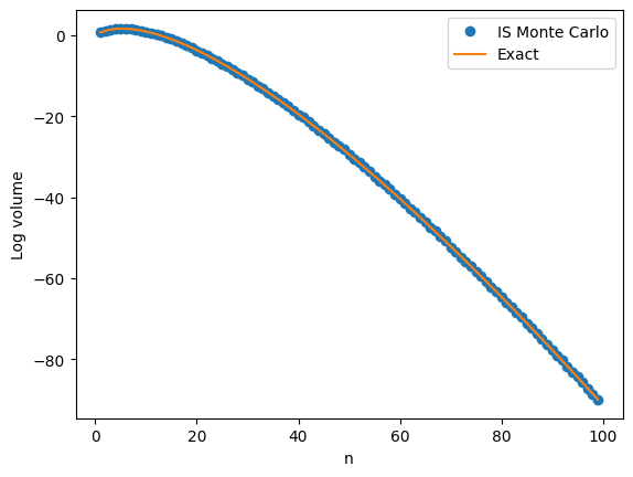
The next plot shows a close agreement between and the IS Monte Carlo approximation on the log scale with going all the way up to .
Notes
There are exact formulas for (available on Wikipedia). I used these to compare the approximations and compute relative errors. There are related problems where no formulas exist and Monte Carlo integration is one of the only ways to get an approximate answer.
The post by John Cook also talks about why the central limit theorem can’t be used to approximate . I initially thought a technique called large deviations could be used to approximate but again this does not directly apply. I was happy to discover that importance sampling worked so well!
The auxiliary variables sampler is a general Markov chain Monte Carlo (MCMC) technique for sampling from probability distributions with unknown normalizing constants [1, Section 3.1]. Specifically, suppose we have functions and we want to sample from the probability distribution That is
where is a normalizing constant. If the set is very large, then it may be difficult to compute or sample from . To approximately sample from we can run an ergodic Markov chain with as a stationary distribution. Adding auxiliary variables is one way to create such a Markov chain. For each , we add a auxiliary variable such that
That is, conditional on , the auxiliary variables are independent and is uniformly distributed on the interval . If is distributed according to and have the above auxiliary variable distribution, then
This means that the joint distribution of is uniform on the set
Put another way, suppose we could jointly sample from the uniform distribution on . Then, the above calculation shows that if we discard and only keep , then will be sampled from our target distribution .
The auxiliary variables sampler approximately samples from the uniform distribution on is by using a Gibbs sampler. The Gibbs samplers alternates between sampling from and then sampling from . Since the joint distribution of is uniform on , the conditional distributions and are also uniform. The auxiliary variables sampler thus transitions from to according to the two step process
Independently sample uniformly from .
Sample uniformly from the set .
Since the auxiliary variables sampler is based on a Gibbs sampler, we know that the joint distribution of will converge to the uniform distribution on . So when we discard , the distribution of will converge to the target distribution !
Auxiliary variables in practice
To perform step 2 of the auxiliary variables sampler we have to be able to sample uniformly from the sets
Depending on the nature of the set and the functions , it might be difficult to do this. Fortunately, there are some notable examples where this step has been worked out. The very first example of auxiliary variables is the Swendsen-Wang algorithm for sampling from the Ising model [2]. In this model it is possible to sample uniformly from . Another setting where we can sample exactly is when is the real numbers and each is an increasing function of . This is explored in [3] where they apply auxiliary variables to sampling from Bayesian posteriors.
There is an alternative to sampling exactly from the uniform distribution on . Instead of sampling uniformly from , we can run a Markov chain from the old that has the uniform distribution as a stationary distribution. This approach leads to another special case of auxiliary variables which is called “slice sampling” [4].
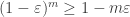
Suppose we have independent events , each of which occur with probability . The event that all of the occur is . By using independence we can calculate the probability of ,
We could also get a lower bound on by using the union bound. This gives,
We can therefore conclude that . This is an instance of Bernoulli’s inequality. More generally, Bernoulli’s inequality states that
for all and . This inequality states the red line is always underneath the black curve in the below picture. For an interactive version of this graph where you can change the value of , click here.
Our probabilistic proof only applies to that case when is between and and is an integer. The more general result can be proved by using convexity. For , the function is convex on the set . The function is the tangent line of this function at the point . Convexity of means that the graph of is always above the tangent line . This tells us that .
For between and , the function is no longer convex but actually concave and the inequality reverses. For , becomes concave again. These two cases are visualized below. In the first picture and the red line is above the black one. In the second picture and the black line is back on top.
Next week I’ll be starting the second year of my statistics PhD. I’ve learnt a lot from taking the first year classes and studying for the qualifying exams. Some of what I’ve learnt has given me a new perspective on some of my old blog posts. Here are three things that I’ve written about before and I now understand better.
1. The Pi-Lambda Theorem
An early post on this blog was titled “A minimal counterexample in probability theory“. The post was about a theorem from the probability course offered at the Australian National University. The theorem states that if two probability measures agree on a collection of subsets and the collection is closed under finite intersections, then the two probability measures agree on the -algebra generated by the collection. In my post I give an example which shows that you need the collection to be closed under finite intersections. I also show that you need to have at least four points in the space to find such an example.
What I didn’t know then is that the above theorem is really a corollary of Dykin’s theorem. This theorem was proved in my first graduate probability course which was taught by Persi Diaconis. Professor Diaconis kept a running tally of how many times we used the theorem in his course and we got up to at least 10. (For more appearances by Professor Diaconis on this blog see here, here and here).
If I were to write the above post again, I would talk about the theorem and rename the post “The smallest -system”. The example given in my post is really about needing at least four points to find a -system that is not a -algebra.
2. Mallow’s Cp statistic
The very first blog post I wrote was called “Complexity Penalties in Statistical Learning“. I wasn’t sure if I would write a second and so I didn’t set up a WordPress account. I instead put the post on the website LessWrong. I no longer associate myself with the rationality community but posting to LessWrong was straight forward and helped me reach more people.
The post was inspired in two ways by the 2019 AMSI summer school. First, the content is from the statistical learning course I took at the summer school. Second, at the career fair many employers advised us to work on our writing skills. I don’t know if would have started blogging if not for the AMSI Summer School.
I didn’t know it at the time but the blog post is really about Mallow’s Cp statistic. Mallow’s Cp statistic is an estimate of the test error of a regression model fit using ordinary least squares. The Mallow’s Cp is equal to the training error plus a “complexity penalty” which takes into account the number of parameters. In the blog post I talk about model complexity and over-fitting. I also write down and explain Mallow’s Cp in the special case of polynomial regression.
In the summer school course I took, I don’t remember the name Mallow’s Cp being used but I thought it was a great idea and enjoyed writing about it. The next time encountered Mallow’s Cp was in the linear models course I took last fall. I was delighted to see it again and learn how it fit into a bigger picture. More recently, I read Brad Efron’s paper “How Biased is the Apparent Error Rate of a Prediction Rule?“. The paper introduces the idea of “effective degrees of freedom” and expands on the ideas behind the Cp statistic.
Incidentally, enrolment is now open for the 2023 AMSI Summer School! This summer it will be hosted at the University of Melbourne. I encourage any Australia mathematics or statistics students reading this to take a look and apply. I really enjoyed going in both 2019 and 2020. (Also if you click on the above link you can try to spot me in the group photo of everyone wearing read shirts!)
3. Finitely additive probability measures
In “Finitely additive measures” I talk about how hard it is to define a finitely additive measure on the set of natural numbers that is not countably additive. In particular, I talked about needing to use the Hahn — Banach extension theorem to extend the natural density from the collection of sets with density to the collection of all subsets of the natural numbers.
There were a number of homework problems in my first graduate probability course that relate to this post. We proved that the sets with density are not closed under finite unions and we showed that the square free numbers have density .
We also proved that any finite measure defined on an algebra of subsets can be extend to the collection of all subsets. This proof used Zorn’s lemma and the resulting measure is far from unique. The use of Zorn’s lemma relates to the main idea in my blog, that defining an additive probability measure is in some sense non-constructive.
Other posts
Going forward, I hope to continue publishing at least one new post every month. I look forward to one day writing another post like this when I can look back and reflect on how much I have learnt.
The material was based on the discussion and references given in this stackexchange post. The title is a reference to a Halloween lecture on measurability given by Professor Persi Diaconis.
What’s scarier than a non-measurable set?
Making every set measurable. Or rather one particular consequence of making every set measurable.
In my talk, I argued that if you make every set measurable, then there exists a set and an equivalence relation on such that . That is, the set has strictly smaller cardinality than the set of equivalence classes . The contradictory nature of this statement is illustrated in the picture below
We can think of the set as the collection of crosses drawn above. The equivalence relation divides into the regions drawn above. The statement means that in some sense there are more regions than crosses.
To make sense of this we’ll first have to be a bit more precise about what we mean by cardinality.
What do we mean by bigger and smaller?
Let and be two sets. We say that and have the same cardinality and write if there exists a bijection function . We can think of the function as a way of pairing each element of with a unique element of such that every element of is paired with an element of .
We next want to define which means has cardinality at most the cardinality of . There are two reasonable ways in which we could try to define this relationship
We could say means that there exists an injective function .
Alternatively, we could means that there exists a surjective function .
Definitions 1 and 2 say similar things and, in the presence of the axiom of choice, they are equivalent. Since we are going to be making every set measurable in this talk, we won’t be assuming the axiom of choice. Definitions 1 and 2 are thus no longer equivalent and we have a decision to make. We will use definition . in this talk. For justification, note that definition 1 implies that there exists a subset such that . We simply take to be the range of . This is a desirable property of the relation and it’s not clear how this could be done using definition 2.
Infinite binary sequences
It’s time to introduce the set and the equivalence relation we will be working with. The set is the set the set of all function . We can think of each elements as an infinite sequence of zeros and ones stretching off in both directions. For example
.
But this analogy hides something important. Each has a “middle” which is the point . For instance, the two sequences below look the same but when we make bold we see that they are different.
,
.
The equivalence relation on can be thought of as forgetting the location . More formally we have if and only if there exists such that for all . That is, if we shift the sequence by we get the sequence . We will use to denote the equivalence class of and for the set of all equivalences classes.
Some probability
Associated with the space are functions , one for each integer . These functions simply evaluate at . That is . A probabilist or statistician would think of as reporting the result of one of infinitely many independent coin tosses. Normally to make this formal we would have to first define a -algebra on and then define a probability on this -algebra. Today we’re working in a world where every set is measurable and so don’t have to worry about -algebras. Indeed we have the following result:
(Solovay, 1970)1There exists a model of the Zermelo Fraenkel axioms of set theory such that there exists a probability defined on all subsets of such that are i.i.d. .
This result is saying that there is world in which, other than the axiom of choice, all the regular axioms of set theory holds. And in this world, we can assign a probability to every subset in a way so that the events are all independent and have probability . It’s important to note that this is a true countably additive probability and we can apply all our familiar probability results to . We are now ready to state and prove the spooky result claimed at the start of this talk.
Proposition: Given the existence of such a probability , .
Proof: Let be any function. To show that we need to show that is not injective. To do this, we’ll first define another function given by . That is, first maps to ‘s equivalence class and then applies to this equivalence class. This is illustrated below.
A commutative diagram showing the definition of as .
We will show that is almost surely constant with respect to . That is, there exists such that . Each equivalence class is finite or countable and thus has probability zero under . This means that if is almost surely constant, then cannot be injective and must map multiple (in fact infinitely many) equivalence classes to .
It thus remains to show that is almost surely constant. To do this we will introduce a third function . The map is simply the shift map and is given by . Note that and are in the same equivalence class for every . Thus, the map satisfies . That is is -invariant.
The map is ergodic. This means that if satisfies , then equals or . For example if is the event that appears at some point in , then and . Likewise if is the event that the relative frequency of heads converges to a number strictly greater than , then and . The general claim that all -invariant events have probability or can be proved using the independence of .
For each , define an event by . Since is -invariant we have that . Thus, or . This gives us a function given by . Note that for every , . This is because if , then , by definition of . Likewise if , then and hence . Thus, in both cases, .
Since is a probability measure, we can conclude that
.
Thus, map to with probability one. Showing that is almost surely constant and hence that is not injective.
There’s a catch!
So we have proved that there cannot be an injective map . Does this mean we have proved ? Technically no. We have proved the negation of which does not imply . To argue that we need to produce a map that is injective. Surprising this is possible and not too difficult. The idea is to find a map such that implies that . This can be done by somehow encoding in where the centre of is.
A simpler proof and other examples
Our proof was nice because we explicitly calculated the value where sent almost all of . We could have been less explicit and simply noted that the function was measurable with respect to the invariant -algebra of and hence almost surely constant by the ergodicity of .
This quicker proof allows us to generalise our “spooky result” to other sets. Below are two examples where
Fix and define if and only if for some .
if and only if .
A similar argument can be used to show that in Solovay’s world . The exact same argument follows from the ergodicity of the corresponding actions on under the uniform measure.
Three takeaways
I hope you agree that this example is good fun and surprising. I’d like to end with some remarks.
The first remark is some mathematical context. This argument given today is linked to some interesting mathematics called descriptive set theory. This field studies the properties of well behaved subsets (such as Borel subsets) of topological spaces. Descriptive set theory incorporates logic, topology and ergodic theory. I don’t know much about the field but in Persi’s Halloween talk he said that one “monster” was that few people are interested in the subject.
The next remark is a better way to think about our “spooky result”. The result is really saying something about cardinality. When we no longer use the axiom of choice, cardinality becomes a subtle concept. The statement no longer corresponds to being “smaller” than but rather that is “less complex” than . This is perhaps analogous to some statistical models which may be “large” but do not overfit due to subtle constraints on the model complexity.
In light of the previous remark, I would invite you to think about whether the example I gave is truly spookier than non-measurable sets. It might seem to you that it is simply a reasonable consequence of removing the axiom of choice and restricting ourselves to functions we could actually write down or understand. I’ll let you decide
Footnotes
Technically Solovay proved that there exists a model of set theory such that every subset of is Borel measurable. To get the result for binary sequences we have to restrict to and use the binary expansion of to define a function . Solvay’s paper is available here https://www.jstor.org/stable/1970696?seq=1


instead of
. ↩︎
![U \in [-1,1]](https://s0.wp.com/latex.php?latex=U+%5Cin+%5B-1%2C1%5D&bg=ffffff&fg=333333&s=0&c=20201002) and
and ![V \in [0,1]](https://s0.wp.com/latex.php?latex=V+%5Cin+%5B0%2C1%5D&bg=ffffff&fg=333333&s=0&c=20201002) are independent and uniformly distributed. Then
are independent and uniformly distributed. Then  has the ratio of uniforms distribution. The plot below shows a histogram based on 10,000 samples from the ratio of uniforms distribution
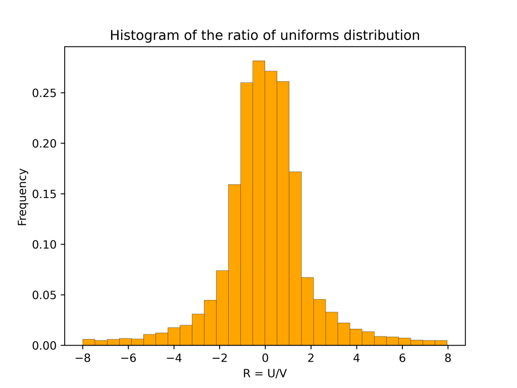
 also has a table mountain shape.


 corresponds to the flat part of the table mountain. The second case corresponds to the sloping curves. The rest of this post use geometry to derive the above formula for
  .
. is uniformly distributed in the box
 ![B=[-1,1] \times [0,1]](https://s0.wp.com/latex.php?latex=B%3D%5B-1%2C1%5D+%5Ctimes+%5B0%2C1%5D&bg=ffffff&fg=333333&s=0&c=20201002) . The image below shows an example of a point
. The image below shows an example of a point  .
.
 and goes through
  . The
. The  .
.
![[R,R+dR]](https://s0.wp.com/latex.php?latex=%5BR%2CR%2BdR%5D&bg=ffffff&fg=333333&s=0&c=20201002) is
is ![\displaystyle{\frac{\text{Area}(\{(u,v) \in B : u/v \in [R, R+dR]\})}{\text{Area}(B)} = \frac{1}{2}\text{Area}(\{(u,v) \in B : u/v \in [R, R+dR]\}).}](https://s0.wp.com/latex.php?latex=%5Cdisplaystyle%7B%5Cfrac%7B%5Ctext%7BArea%7D%28%5C%7B%28u%2Cv%29+%5Cin+B+%3A+u%2Fv+%5Cin+%5BR%2C+R%2BdR%5D%5C%7D%29%7D%7B%5Ctext%7BArea%7D%28B%29%7D+%3D+%5Cfrac%7B1%7D%7B2%7D%5Ctext%7BArea%7D%28%5C%7B%28u%2Cv%29+%5Cin+B+%3A+u%2Fv+%5Cin+%5BR%2C+R%2BdR%5D%5C%7D%29.%7D&bg=ffffff&fg=333333&s=0&c=20201002)
![\displaystyle{h(R) = \lim_{dR \to 0} \frac{1}{2dR}\text{Area}(\{(u,v) \in B : u/v \in [R, R+dR]\})}.](https://s0.wp.com/latex.php?latex=%5Cdisplaystyle%7Bh%28R%29+%3D+%5Clim_%7BdR+%5Cto+0%7D+%5Cfrac%7B1%7D%7B2dR%7D%5Ctext%7BArea%7D%28%5C%7B%28u%2Cv%29+%5Cin+B+%3A+u%2Fv+%5Cin+%5BR%2C+R%2BdR%5D%5C%7D%29%7D.&bg=ffffff&fg=333333&s=0&c=20201002)
 and
and  . In this case, the set
 ![\{(u,v) \in B : u/v \in [R, R+dR]\}](https://s0.wp.com/latex.php?latex=%5C%7B%28u%2Cv%29+%5Cin+B+%3A+u%2Fv+%5Cin+%5BR%2C+R%2BdR%5D%5C%7D&bg=ffffff&fg=333333&s=0&c=20201002) is a triangle. This triangle is drawn in blue below.
is a triangle. This triangle is drawn in blue below.
 . The perpendicular height of the triangle from the horizontal edge is
 ![\displaystyle{\text{Area}(\{(u,v) \in B : u/v \in [R, R+dR]\}) =\frac{1}{2}\times dR \times 1=\frac{dR}{2}}.](https://s0.wp.com/latex.php?latex=%5Cdisplaystyle%7B%5Ctext%7BArea%7D%28%5C%7B%28u%2Cv%29+%5Cin+B+%3A+u%2Fv+%5Cin+%5BR%2C+R%2BdR%5D%5C%7D%29+%3D%5Cfrac%7B1%7D%7B2%7D%5Ctimes+dR+%5Ctimes+1%3D%5Cfrac%7BdR%7D%7B2%7D%7D.&bg=ffffff&fg=333333&s=0&c=20201002)
![R \in [-1,1]](https://s0.wp.com/latex.php?latex=R+%5Cin+%5B-1%2C1%5D&bg=ffffff&fg=333333&s=0&c=20201002) we have
we have

 . The perpendicular height of the triangle from the vertical edge is
 ![\displaystyle{\text{Area}(\{(u,v) \in B : u/v \in [R, R+dR]\}) =\frac{1}{2}\times \frac{dR}{R(R+dR)} \times 1=\frac{dR}{2R(R+dR)}}.](https://s0.wp.com/latex.php?latex=%5Cdisplaystyle%7B%5Ctext%7BArea%7D%28%5C%7B%28u%2Cv%29+%5Cin+B+%3A+u%2Fv+%5Cin+%5BR%2C+R%2BdR%5D%5C%7D%29+%3D%5Cfrac%7B1%7D%7B2%7D%5Ctimes+%5Cfrac%7BdR%7D%7BR%28R%2BdR%29%7D+%5Ctimes+1%3D%5Cfrac%7BdR%7D%7B2R%28R%2BdR%29%7D%7D.&bg=ffffff&fg=333333&s=0&c=20201002)

 and
and  . This is because the ratio of uniform distribution has heavy tails. This meant that there were some very large values of
  . It is a u-shaped distribution. There are peaks at
  and
and  and a dip in the middle. The figure below shows the probability distribution function for
  .
.

 is distributed according to the discrete arcsine distribution with parameter
  converges in distribution to the continuous arcsine distribution on
 ![[0,1]](https://s0.wp.com/latex.php?latex=%5B0%2C1%5D&bg=ffffff&fg=333333&s=0&c=20201002) . The continuous arcsine distribution has the probability density function
. The continuous arcsine distribution has the probability density function
 . It is called the arcsine distribution because the cumulative distribution function involves the arcsine function
 . I was surprised when I was told this, and couldn’t find a reference. The rest of this blog post proves that the discrete arcsine distribution is an instance of the beta-binomial distribution.
 is the Beta-function. To show that the discrete arc sine distribution is an instance of the beta-binomial distribution we need that
  . That is
 ,
, . To prove the above equation, we can first do some simplifying to
  . By definition
 ,
, factorial if
  is a natural number. The Gamma function
  also satisfies the property
 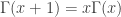 . Using this repeatedly gives

 is the double factorial. The same reasoning gives

 is also equal to the above final expression. Recall
 (and hence
  ). To see why this last claim holds, note that
 as claimed.
 samples to estimate
  , the volume of an

 .
. . That is the distribution
  is an
is an  . The conditional target distribution is
  the uniform distribution on the
  . Here
  is the Kullback-Liebler divergence between
  . Kullback-Liebler divergence is defined as integral. Specifically
 to be the distribution of the norm squared under
  , then
  and likewise for
  . By the rotational symmetry of
 and
and ![r \in [0,1]](https://s0.wp.com/latex.php?latex=r+%5Cin+%5B0%2C1%5D&bg=ffffff&fg=333333&s=0&c=20201002)

 . This means that
  . The distribution
  , then
  is a scaled chi-squared variable. The shape parameter of
  . The density for


 we get that for large
  .
.
 are independent and uniformly distributed on the interval
 ![[-1,1]](https://s0.wp.com/latex.php?latex=%5B-1%2C1%5D&bg=ffffff&fg=333333&s=0&c=20201002) then
then
 with
with  uniform on
  . Next, we count the proportion of vectors
  with
with  . Specifically, if
  is equal to one when

 and the Monte Carlo approximation with
  .
. is even smaller! For example when
  ,
,  . This means that in our one thousand samples we only expect two or three occurrences of the event
  . As a result our estimate has a high variance.
 , the relative error in the approximation is 100%.
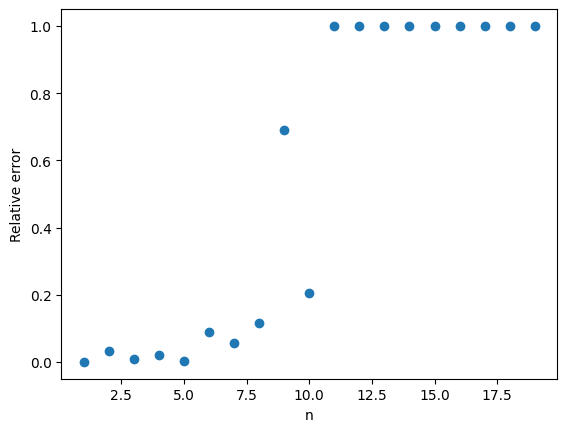
 from the uniform distribution on
  becomes more likely.
 , we give weights to each of samples and then add up the weights.
  is the density of the proposal distribution, then the IS Monte Carlo estimate of
 and
and  implies
  , the IS Monte Carlo estimate will be an unbiased estimate of
  is one and so the event
 .
.
 and we want to sample from the probability distribution
  That is
 is a normalizing constant. If the set
  is very large, then it may be difficult to compute
  or sample from
  . To approximately sample from
  , we add a auxiliary variable
  such that
 ![\displaystyle{P(U \mid X) = \prod_{i=1}^n \mathrm{Unif}[0,f_i(X)]}.](https://s0.wp.com/latex.php?latex=%5Cdisplaystyle%7BP%28U+%5Cmid+X%29+%3D+%5Cprod_%7Bi%3D1%7D%5En+%5Cmathrm%7BUnif%7D%5B0%2Cf_i%28X%29%5D%7D.&bg=ffffff&fg=333333&s=0&c=20201002)
 are independent and
  is uniformly distributed on the interval
 ![[0,f_i(X)]](https://s0.wp.com/latex.php?latex=%5B0%2Cf_i%28X%29%5D&bg=ffffff&fg=333333&s=0&c=20201002) . If
. If ![\displaystyle{P(X,U) =P(X)P(U\mid X)\propto \prod_{i=1}^n f_i(X) \frac{1}{f_i(X)} I[U_i \le f(X_i)] = \prod_{i=1}^n I[U_i \le f(X_i)]}.](https://s0.wp.com/latex.php?latex=%5Cdisplaystyle%7BP%28X%2CU%29+%3DP%28X%29P%28U%5Cmid+X%29%5Cpropto++%5Cprod_%7Bi%3D1%7D%5En+f_i%28X%29+%5Cfrac%7B1%7D%7Bf_i%28X%29%7D+I%5BU_i+%5Cle+f%28X_i%29%5D+%3D+%5Cprod_%7Bi%3D1%7D%5En+I%5BU_i+%5Cle+f%28X_i%29%5D%7D.&bg=ffffff&fg=333333&s=0&c=20201002)
 is uniform on the set
 . Then, the above calculation shows that if we discard
  and only keep
  from
from  and then sampling
  from
from  . Since the joint distribution of
  and
and  .
.
 , it might be difficult to do this. Fortunately, there are some notable examples where this step has been worked out. The very first example of auxiliary variables is the Swendsen-Wang algorithm for sampling from the Ising model [2]. In this model it is possible to sample uniformly from
  . Another setting where we can sample exactly is when
  and each
  , each of which occur with probability
  . The event that all of the
  occur is
  . By using independence we can calculate the probability of
  ,
,
 by using the union bound. This gives,
 . This is an instance of
 and
and  . This inequality states the red line is always underneath the black curve in the below picture. For an interactive version of this graph where you can change the value of
 is between
  is convex on the set
  . The function
  is the tangent line of this function at the point
  . Convexity of
  . This tells us that
  .
.  is no longer convex but actually concave and the inequality reverses. For
  ,
,  and the red line is above the black one. In the second picture
  and the black line is back on top.

 -algebra generated by the collection. In my post I give an example which shows that you need the collection to be closed under finite intersections. I also show that you need to have at least four points in the space to find such an example.
 .
. 
 and an equivalence relation
  on
on  . That is, the set
  . The contradictory nature of this statement is illustrated in the picture below
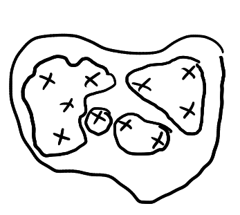
 means that in some sense there are more regions than crosses.
 and
and  if there exists a bijection function
  . We can think of the function
  as a way of pairing each element of
  which means
  .
. .
. such that
  . We simply take
  to be the range of
  the set of all function
  . We can think of each elements
  as an infinite sequence of zeros and ones stretching off in both directions. For example
 .
. . For instance, the two sequences below look the same but when we make
  ,
, .
. if and only if there exists
  such that
  for all
  . That is, if we shift the sequence
  by
by  . We will use
 ![[\omega]](https://s0.wp.com/latex.php?latex=%5B%5Comega%5D&bg=ffffff&fg=333333&s=0&c=20201002) to denote the equivalence class of
to denote the equivalence class of  , one for each integer
  . That is
  . A probabilist or statistician would think of
  as reporting the result of one of infinitely many independent coin tosses. Normally to make this formal we would have to first define a
  defined on all subsets of
  .
. in a way so that the events
  are all independent and have probability
  . It’s important to note that this is a true countably additive probability and we can apply all our familiar probability results to
  .
. be any function. To show that
  given by
 ![g(\omega)=f([\omega])](https://s0.wp.com/latex.php?latex=g%28%5Comega%29%3Df%28%5B%5Comega%5D%29&bg=ffffff&fg=333333&s=0&c=20201002) . That is,
. That is,  first maps
 is almost surely constant with respect to
  such that
  . Each equivalence class
  .
. is almost surely constant. To do this we will introduce a third function
  . The map
  is simply the shift map and is given by
  . Note that
  are in the same equivalence class for every
  . Thus, the map
  . That is
  , then
  equals
  appears at some point in
  . Likewise if
  . The general claim that all
  by
by  . Since
  . Thus,
  or
or  given by
  . Note that for every
  . This is because if
  , then
  , by definition of
  . Likewise if
  , then
  and hence
  . Thus, in both cases,
  .
. .
.
 . Does this mean we have proved
  ? Technically no. We have proved the negation of
  which does not imply
  . To argue that
  that is injective. Surprising this is possible and not too difficult. The idea is to find a map
  implies that
  . This can be done by somehow encoding in
  where the centre of
 and define
  for some
  .
. is Borel measurable. To get the result for binary sequences we have to restrict to
  and use the binary expansion of
  to define a function
  . Solvay’s paper is available here