Two weeks ago I gave talk titled “Two Combings of  “. The talk was about some material I have been discussing lately with my honours supervisor. The talk went well and I thought it would be worth sharing a written version of what I said.
Geometric Group Theory
Combings are a tool that gets used in a branch of mathematics called geometric group theory. Geometric group theory is a relatively new area of mathematics and is only around 30 years old. The main idea behind geometric group theory is to use tools and ideas from geometry and low dimensional topology to study and understand groups. It turns out that some of the simplest questions one can ask about groups have interesting geometric answers. For instance, the Dehn function of a group gives a natural geometric answer to the solvability of the word problem.
Generators
Before we can define what a combing is we’ll need to set up some notation. If  is a set then we will write
  for the set of words written using elements of and inverses of elements of . For instance if
  , then
  (here
(here  refers to the empty word). If
  is a word in , we will write
  for the length of . Thus
  and so on.
If  is a group and is a subset of , then we have a natural map
  given by:
 .
.
We will say that generates if the above map is surjective. In this case we will write  for
for  when is a word in .
The Word Metric
The geometry in “geometric group theory” often arises when studying how a group acts on different geometric spaces. A group always acts on itself by left multiplication. The following definition adds a geometric aspect to this action. If is a group with generators , then the word metric on with respect to is the function  given by

That, is the distance between two group elements  is the length of the shortest word in we can use to represent
  . Equivalently the distance between
  and
and  is the length of the shortest word we have to append to to produce . This metric is invariant under left-multiplication by (ie
  for all
  ). Thus acts on
  by isometries.
Words are Paths
Now that we are viewing the group as a geometric space, we can also change how we think of words  . Such a word can be thought of as discrete path in . That is we can think of as a function from
  to . This way of thinking of as a discrete path is best illuminated with an example. Suppose we have the word
  , then


 .
.
Thus the path  is given by taking the first
  letters of and mapping this word to the group element it represents. With this interpretation of word in in mind we can now define combings.
Combings
Let be a group with a finite set of generators . Then a combing of with respect to is a function  such that
- For all
 ,
,  (we will write
  for
for  .
. - There exists
 such that for all
  with
with  for some
  , we have that
  for all
  .
.
The first condition says that we can think of  as a way of picking a normal form
  for each . The second condition is a bit more involved. It states that if the group elements are distance 1 from each other in the word metric, then the paths
  are within distance
  of each other at any point in time.
An Example
Not all groups can be given a combing. Indeed if we have a combing of , then the word problem in is solvable and the Dehn function of is at most exponential. One group that does admit a combing is  . This group is generated by
  and one combing of with respect to this generating set is
 .
.
The first condition of being a combing is clearly satisfied and the following picture shows that the second condition can be satisfied with  .
.
A Non-Example
The discrete Heisenberg group,  , can be given by the following presentation
 .
.
That is, the group has three generators  and
and  . The generator commutes with both
  and
and  . The generators and almost commute but don’t quite as seen in the relation
  .
.
Any  can be represented uniquely as
  for
for  . To see why such a representation exists it’s best to consider an example. Suppose that
  . Then we can use the fact that commutes with and to push all ‘s to the right and we get that
  . We can then apply the third relation to switch the order of and on the right. This gives us that that
  . If we apply this relation once more we get that
  and thus
  . The procedure used to write in the form
  can be generalized to any word written using
  .
.
The fact the such a representation is unique (that is if  , then
  ) is harder to justify but can be proved by defining an action of on
  . Thus we can define a function
  by setting
  to be the unique word of the form
  that represents . This map satisfies the first condition of being a combing and has many nice properties. These include that it is easy to check whether or not a word in
  is equal to for some and there are fast algorithms for putting a word in into its normal form. Unfortunately this map fails to be a combing.
The reason why fails to be a combing can be seen back when we turned  into
into  . To move ‘s on the right to the left we had to move past ‘s and produce ‘s in the process. More concretely fix
  and let
  and
and  . We have
  and
and  . The group elements and differ by a generator. Thus, if was a combing we should be able to uniformly bound
  for all and all .
If we then let  , we can recall that

We have that  and
and  and thus

The group element  cannot be represented as a shorter element of and thus
  and the map
  is not a combing.
Can we comb the Heisenberg group?
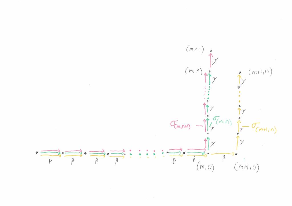
This leaves us with a question, can we comb the group ? It turns out that we can but the answer actually lies in finding a better combing of . This is because contains the subgroup  . Rather than using the normal form
  , we will use
  where
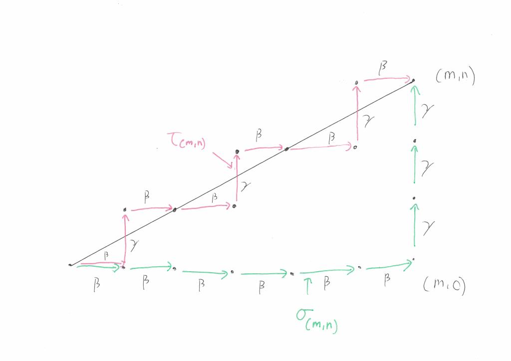
where  is a combing of that is more symmetric. The word
  is defined to be the sequence of
  ‘s and
  ‘s that stays closest to the straight line in
  that joins
  to
to  (when we view and as representing
  and
and  respectively). Below is an illustration:
This new function isn’t quite a combing of but it is the next best thing! It is an asynchronous combing. An asynchronous combing is one where we again require that the paths  stay close to each other whenever and are close to each other. However we allow the paths and to travel at different speeds. Many of the results that can be proved for combable groups extend to asynchronously combable groups.
References
Hairdressing in Groups by Sarah Rees is a survey paper that includes lots examples of groups that do or do not admit combings. It also talks about the language complexity of a combing, something I didn’t have time to touch on in my talk.
Combings of Semidirect Products and 3-Manifold Groups by Martin Bridson contains a proof that is asynchornously combable. He actually proves the more general result that any group of the form  is asynchronously combable.
Thank you to my supervisor, Tony Licata, for suggesting I give my talk on combing and for all the support he has given me so far.


-measurable.
,
, where
is the indicator function of
.

![[-1,1]^2 \subseteq \mathbb{R}^2](https://s0.wp.com/latex.php?latex=%5B-1%2C1%5D%5E2+%5Csubseteq+%5Cmathbb%7BR%7D%5E2&bg=ffffff&fg=333333&s=0&c=20201002)


![A\subseteq [-1,1]](https://s0.wp.com/latex.php?latex=A%5Csubseteq+%5B-1%2C1%5D&bg=ffffff&fg=333333&s=0&c=20201002)


![V \in [-\sqrt{1-U^2}, \sqrt{1-U^2}]](https://s0.wp.com/latex.php?latex=V+%5Cin+%5B-%5Csqrt%7B1-U%5E2%7D%2C+%5Csqrt%7B1-U%5E2%7D%5D&bg=ffffff&fg=333333&s=0&c=20201002)
![\mathbb{E}[X1_B] = \int_A \int_{-\sqrt{1-u^2}}^{\sqrt{1-u^2}} \frac{1}{4}dvdu = \int_A \frac{1}{2}\sqrt{1-u^2}du](https://s0.wp.com/latex.php?latex=%5Cmathbb%7BE%7D%5BX1_B%5D+%3D+%5Cint_A+%5Cint_%7B-%5Csqrt%7B1-u%5E2%7D%7D%5E%7B%5Csqrt%7B1-u%5E2%7D%7D+%5Cfrac%7B1%7D%7B4%7Ddvdu+%3D+%5Cint_A+%5Cfrac%7B1%7D%7B2%7D%5Csqrt%7B1-u%5E2%7Ddu&bg=ffffff&fg=333333&s=0&c=20201002)
![[-1,1]](https://s0.wp.com/latex.php?latex=%5B-1%2C1%5D&bg=ffffff&fg=333333&s=0&c=20201002)
![\frac{1}{2}1_{[-1,1]}](https://s0.wp.com/latex.php?latex=%5Cfrac%7B1%7D%7B2%7D1_%7B%5B-1%2C1%5D%7D&bg=ffffff&fg=333333&s=0&c=20201002)
![\mathbb{E}[Y1_B] = \mathbb{E}[\sqrt{1-U^2}1_{\{U \in A\}}] = \int_A \frac{1}{2}\sqrt{1-u^2}du](https://s0.wp.com/latex.php?latex=%5Cmathbb%7BE%7D%5BY1_B%5D+%3D+%5Cmathbb%7BE%7D%5B%5Csqrt%7B1-U%5E2%7D1_%7B%5C%7BU+%5Cin+A%5C%7D%7D%5D+%3D+%5Cint_A+%5Cfrac%7B1%7D%7B2%7D%5Csqrt%7B1-u%5E2%7Ddu&bg=ffffff&fg=333333&s=0&c=20201002)
![\mathbb{E}[X1_B] = \mathbb{E}[Y1_B]](https://s0.wp.com/latex.php?latex=%5Cmathbb%7BE%7D%5BX1_B%5D+%3D+%5Cmathbb%7BE%7D%5BY1_B%5D&bg=ffffff&fg=333333&s=0&c=20201002)

![V \in [-\sqrt{1-u^2},\sqrt{1+u^2}]](https://s0.wp.com/latex.php?latex=V+%5Cin+%5B-%5Csqrt%7B1-u%5E2%7D%2C%5Csqrt%7B1%2Bu%5E2%7D%5D&bg=ffffff&fg=333333&s=0&c=20201002)

![[-\sqrt{1-u^2},\sqrt{1+u^2}]](https://s0.wp.com/latex.php?latex=%5B-%5Csqrt%7B1-u%5E2%7D%2C%5Csqrt%7B1%2Bu%5E2%7D%5D&bg=ffffff&fg=333333&s=0&c=20201002)

![f:[-1,1]\to \mathbb{R}](https://s0.wp.com/latex.php?latex=f%3A%5B-1%2C1%5D%5Cto+%5Cmathbb%7BR%7D&bg=ffffff&fg=333333&s=0&c=20201002)
![f(x) \in [0,1]](https://s0.wp.com/latex.php?latex=f%28x%29+%5Cin+%5B0%2C1%5D&bg=ffffff&fg=333333&s=0&c=20201002)
![A \subseteq [-1,1]^2](https://s0.wp.com/latex.php?latex=A+%5Csubseteq+%5B-1%2C1%5D%5E2&bg=ffffff&fg=333333&s=0&c=20201002)

 and
and  , a coupling of
  on
on  where
where  has the same distribution as
  has the same distribution as
  .
. where
where  . This coupling corresponds to a random vector
  where
where  and
and  are independent and (as is required for all couplings)
  ,
,  .
.  is in the “middle” of all couplings. This is because
 ![H_L, H_U :\mathbb{R}^2 \to [0,1]](https://s0.wp.com/latex.php?latex=H_L%2C+H_U+%3A%5Cmathbb%7BR%7D%5E2+%5Cto+%5B0%2C1%5D&bg=ffffff&fg=333333&s=0&c=20201002) by
by and
and  .
. and
and  are distributions functions on
  and
and  .
. and
and  be the quantile functions of
  and
and  .
.![[0,1]](https://s0.wp.com/latex.php?latex=%5B0%2C1%5D&bg=ffffff&fg=333333&s=0&c=20201002) and define
and define and
and  .
. if and only if
  , we have
  and likewise
  . Furthermore
  occurs if and only if
  which is equivalent to
  . Thus
 is distributed according to
  and
and  are closely related as they are both increasing functions of a common random variable
  and
and  .
. and
and  are again functions of a common random variable
  is also uniformly distributed on
  and
and  .
.  occurs if and only if
  which occurs if and only if
  . If
. If  , then
  and
and  . On the other hand, if
  , then
  and
and  . Thus
 ,
, is distributed according to
  , we can look at the quantity
 would be positive and if
  , the quantity
  and it is in this sense that they are extremal. This final claim is the two dimensional version of
  be a set and let
  be a
be a  be a function with the following properties
 .
. in
in  , we have
  .
. is a sequence of sets in
  for all
  and
and  , then, as
  .
.  is a probability measure on
  . This amounts to showing that
  is a sequence of pairwise disjoint sets, then
  . One way to do this is define
  . Since the sets
  as
as  .
. . Thus by applying the second property of
  .
. and let
  is to look at the proportion of elements in
 . More generally if
  . The function
  .
. be a finite collection of disjoint subsets of
  . Then for every natural number
  .
. .
. , as required. Furthermore, the function
  for each
  . Then
  and
and  . On the other hand
  for every
  .
. does not always exist. Consider the set
  , ie a number
  is in
is in  for some odd number
  . The idea with the set
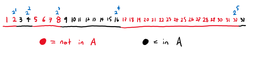
 represent the sequence of numbers
  , then
  , then
  or
or  we can calculate exactly what
  .
. and
and  we have
 .
. and
and 
 and
and  . Thus the limit of
  ,
, is now a Banach limit. This new definition of
  and you write
  where each
  and
and  is a prime number, then in fact
  and we wrote the same prime numbers (but maybe in a different order).
  . People in this world can add numbers and multiply numbers just like we can. They can even talk about divisibility, for example
  divides
  since
since  . Note that things are already getting a bit strange in this world. Since there is no number one, numbers in this world do not divide themselves.
 is also prime in this world. This is because there are no two even numbers that multiply together to make
  and
and  such that
  . Since
  and
and  can be factorized uniquely.
 can be factorized uniquely.
 is prime.
 can be factorized uniquely.
 is prime.
 can be factorized uniquely.
 is prime.
 can be factorized uniquely.
 and we have:
 and
and  .
. where
where  and
and  are both integers. One way to try to solve this is by rewriting the equation as
  . With this rewriting we have left the familiar world of the whole numbers and entered the number ring
 ![\mathbb{Z}[\sqrt{-19}]](https://s0.wp.com/latex.php?latex=%5Cmathbb%7BZ%7D%5B%5Csqrt%7B-19%7D%5D&bg=ffffff&fg=333333&s=0&c=20201002) .
.  , where
  .
. . Thus
 .
. , then
  and
and  are coprime in
  is a cube and if two coprime numbers multiply to be a cube, then both of those coprime numbers must be cubes.
 . If we expand out this cube we can conclude that
 .
. . This implies that
  and
and  . Hence
  and
and  . Now if
  , then
  – a contradiction. Similarly if
  , then
  – another contradiction. Thus we can conclude there are no integer solutions to the equation
  . Thus simply assuming that that the ring
  have the same cardinality. That is the set of all non-negative integers
  has the same size as the set of all pairs on non-negative integers
  , or put less precisely “infinity times infinity equals infinity”.
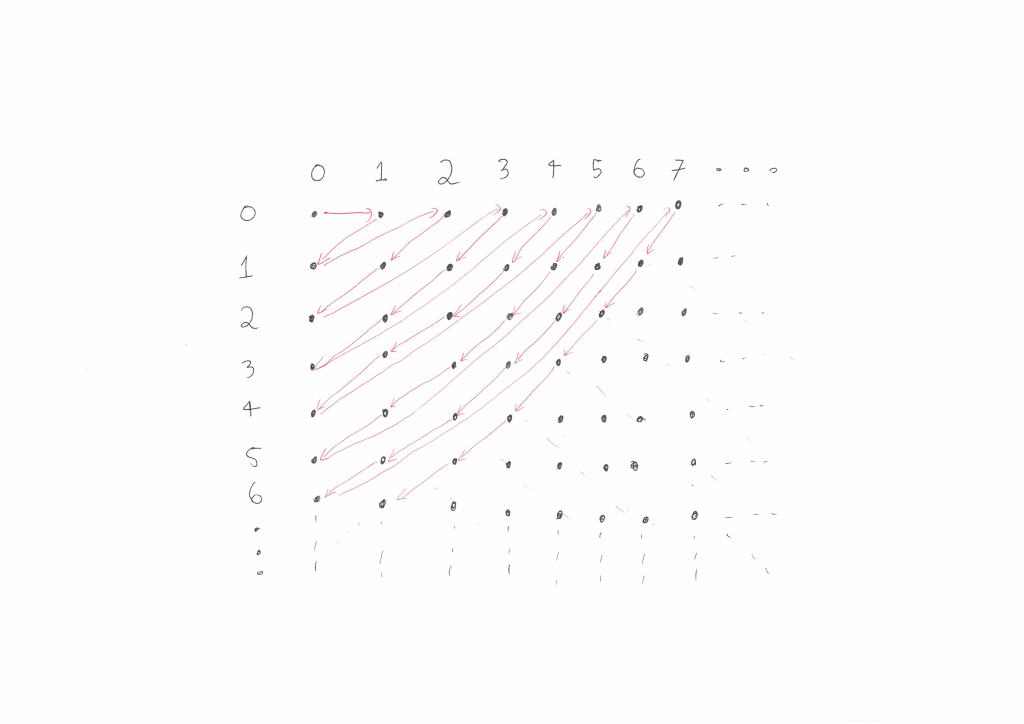
  . We will call such a function a pairing function since it takes in two numbers and pairs them together to create a single number. An example of one such function is


 , first find the dot that
  as a path in the grid. This is done by starting at
  and joining
  to
to  . It’s a fun exercise to work out what the path corresponding to
  . When represented as a path, this is what
 , then the value of
  is
is  . This is because to get to
  , we have to go along
  . The above path first goes through
 . That is the function
  . When thinking of pairing functions as paths in a grid, this transformation amounts to reflecting the picture along the diagonal
  .
. 
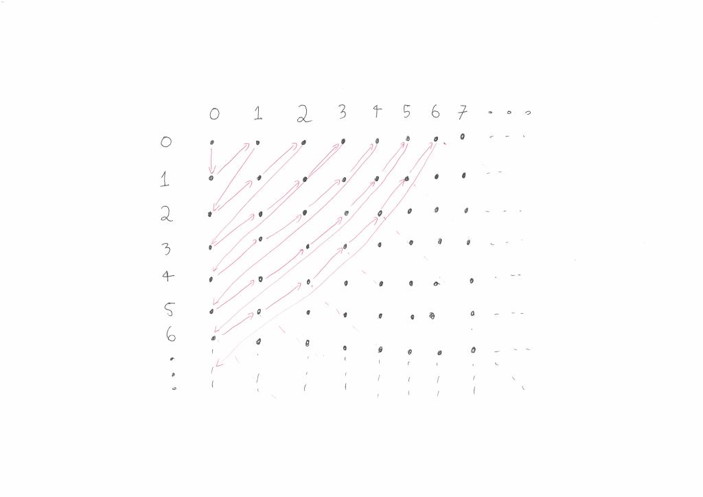
 . The Fueter–Pólya theorem states these two are actually the only quadratic pairing functions! In fact it is conjectured that these two quadratics are the only polynomial pairing functions but this is still an open question.
 where:
 and
and  and hence
  .
.![\mathbb{P}: \mathcal{F} \rightarrow [0,1]](https://s0.wp.com/latex.php?latex=%5Cmathbb%7BP%7D%3A+%5Cmathcal%7BF%7D+%5Crightarrow+%5B0%2C1%5D&bg=ffffff&fg=333333&s=0&c=20201002) such that
such that  and for all countable collections
  of mutually disjoint subsets we have that
  .
. and
and  which is the smallest
 that contain
 ![\mathbb{P}_0 : \mathcal{G} \rightarrow [0,1]](https://s0.wp.com/latex.php?latex=%5Cmathbb%7BP%7D_0+%3A+%5Cmathcal%7BG%7D+%5Crightarrow+%5B0%2C1%5D&bg=ffffff&fg=333333&s=0&c=20201002) and we want to extend this function to create a probability measure
and we want to extend this function to create a probability measure ![\mathbb{P} : \sigma(\mathcal{G}) \rightarrow [0,1]](https://s0.wp.com/latex.php?latex=%5Cmathbb%7BP%7D+%3A+%5Csigma%28%5Cmathcal%7BG%7D%29+%5Crightarrow+%5B0%2C1%5D&bg=ffffff&fg=333333&s=0&c=20201002) . A
. A  on
on  but
but  ? The following theorem gives a criterion that guarantees no such
 ![\mathbb{P},\mathbb{P}' : \sigma(\mathcal{G}) \rightarrow [0,1]](https://s0.wp.com/latex.php?latex=%5Cmathbb%7BP%7D%2C%5Cmathbb%7BP%7D%27+%3A+%5Csigma%28%5Cmathcal%7BG%7D%29+%5Crightarrow+%5B0%2C1%5D&bg=ffffff&fg=333333&s=0&c=20201002) are two probability measures such that
are two probability measures such that  , then
  .
. but
but  . We will however have
  and thus we might be able to find two probability measure
  and
and  but
but  . The following counterexample shows that this intuition is indeed well-founded.
![\mathbb{P}: \sigma(\mathcal{G}) \rightarrow [0,1]](https://s0.wp.com/latex.php?latex=%5Cmathbb%7BP%7D%3A+%5Csigma%28%5Cmathcal%7BG%7D%29+%5Crightarrow+%5B0%2C1%5D&bg=ffffff&fg=333333&s=0&c=20201002) can be defined by specifying the values
can be defined by specifying the values  for each
  .
. such that
  is not equal to
  or
or  .
.  . Up to relabelling the elements of
  . This has a chance of working since
  must satisfy the equations
 ,
, ,
, .
. ,
,  and
and  . Thus
  and
and  .
. is sufficient for our counter example! We can let
  . Then
  and we can define
 ![\mathbb{P} , \mathbb{P}' : \sigma (\mathcal{G}) \rightarrow [0,1]](https://s0.wp.com/latex.php?latex=%5Cmathbb%7BP%7D+%2C+%5Cmathbb%7BP%7D%27+%3A+%5Csigma+%28%5Cmathcal%7BG%7D%29+%5Crightarrow+%5B0%2C1%5D&bg=ffffff&fg=333333&s=0&c=20201002) by
by ,
,  ,
,  and
and  .
. ,
,  ,
,  and
and  .
.  and
and  . Thus we have our counterexample! In general for any
  we can define the probability measure
  . The measure
  is not equal to